Record what I have learnt from the beginning.
As there are very few solutions on how to utilize GPU without CUDA, we will use cudatoolkit with approprivate version of cudnn. There are two ways to meet this requirement: First install the nvidia graphic card driver, then:
-
Scroll to the bottom of official list and download+install the corresponding version of cudatoolkit + cudnn. Advantange of doing this is: you can try the latest version of tensorflow-gpu which can be pip-installed from the bottom list of here; or
-
Upon downloading the card driver, just use conda install tensorflow-gpu, it will automatically download the cudatoolkit and cudnn for you inside your activated conda environment. Usually the conda cloud version of tensorflow-gpu lags behind the official latest version.
-
to close
I Tensorflow/...logs, we useTF_CPP_MIN_LOG_LEVEL=1Here is the meaning of levels 0, 1, 2, 3:
0 = all messages are logged (default behavior)
1 = INFO messages are not printed
2 = INFO and WARNING messages are not printed
3 = INFO, WARNING, and ERROR messages are not printed
Things start to be confusing when we deal with dataset with different purposes:
LabelEncoderturns our array of classes into array of integers, i.e., array of binarized labels.LabelBiniarizerturns our array of classes into array of probability vectors, each has only 1 nonzero entry.
We will save our binaized label into an hdf5 dataset file, via tensorflow.keras.utils.to_categorical we then turn them into probability vector when generating dataset.
Implemented the whole back-prop update process from scratch. The back-propagation formula is based on calculating at the
-th layer, and passing it to the
-th layer with the following formula:

Derivations of this formular is recorded in my blog post:
Study how to train a model to draw bounding box of specific object.

One Conv layer structure for identifying animals of 3 classes. Also learn how to serialize my model and load my trained weights. Average accuracy is just about 70%. study purpose.
Implement LeNet and train it through the mnist dataset of 0-9.
Implement a similified version of VGG Net and trained using CIFAR-10 dataset. Added dropout layer, added momentum and nesterov acceleration in SGD. Also introduce BatchNormalization to see difference.
-
We introduce learning rate decay per iteration in kwarg of
SGD. The built-in decay formula ofSGDis given by:The validation accuracy is about 0.82, its loss, val_loss, accuracy and val_accuracy are plotted in output/cifar10_minivggnet.png.
-
We also try to introduce a learning rate decay per 5 epochs by providing a callback function in kwarg of
model.fit. The decay factor is set to 0.25 to observe what happens when learning rate decays too quickly, resulting in stagnant decrease in both training and validation loss (see output/cifar10_lr_decay_f0.25_plot.png) -
We introduce a callback function class,
TrainingMonitorCallback, which extendsBaseLoggerfromkeras.callbacks. We override theon_epoch_endmethod and plot the graph of loss, val_loss, accuracy, val_accuracy once an epoch ends (I have plotted 43 of them, see output for detail). The learning rate is constantly 0.01 without decay as a baseline to see if we should further apply regularization process. -
We import
ModelCheckpointfromkeras.callbacksand define a template string to save various weights when validation loss decreases. We can get the smallest one without redundant files by simply removing the template part infname. -
To run this script we will need to install graphviz and pydot on mac:
brew install graphviz && pip install graphviz && pip install pydotThis package is to visualize our model to check if there is any faulty design like incorrect calculation of output shape. For example, our MiniVGGNet is visualized in here.
-
- Dropout on convolutional layers is weird
- Deep learning for pedestrians: backpropagation in CNNs
- Batch Normalization: Accelerating Deep Network Training by Reducing Internal Covariate Shift
- Andrew Ng's Gradient Descent With Momentum (C2W2L06) video
- 機器/深度學習-基礎數學(三):梯度最佳解相關算法(gradient descent optimization algorithms)
Make prediction using pre-trained model (with weights being trained from ImageNet). The following script in console will do:
python imagenet_pretrained.py --image example_images/example_01.jpg --model vgg16
A full description of 3 image preprocessings given by Keras:
In case we have difficulty choosing python interpretor in mac (and in case we are not using a pipenv):
We study the effect of data augmentation. We train our miniVGGNet on flower-17 dataset. The dataset has 80 images in each of 17 classes, which is usually considered "not enough" for classification problem. Without augmentation, we see the evidence of overfitting very quickly from here at the 20-th epoch. Its classification report on test set is:
-
Click me to show validation accuracy without data augmentation
            precision    recall  f1-score   support

  Bluebell       0.61      0.69      0.65        16
 Buttercup       0.59      0.67      0.62        15
Colts'Foot       0.43      0.45      0.44        20
   Cowslip       0.30      0.50      0.37        18
    Crocus       0.65      0.52      0.58        21
  Daffodil       0.22      0.17      0.20        23
     Daisy       0.70      0.61      0.65        23
Dandeilion       0.52      0.67      0.59        18
Fritillary       0.80      0.84      0.82        19
      Iris       0.94      0.79      0.86        19
LilyValley       0.46      0.60      0.52        20
     Pansy       0.84      0.59      0.70        27
  Snowdrop       0.31      0.23      0.26        22
 Sunflower       0.86      0.83      0.84        23
 Tigerlily       0.74      0.88      0.80        16
     Tulip       0.35      0.35      0.35        20
Windflower       0.56      0.50      0.53        20

  accuracy                           0.57       340
 macro avg       0.58      0.58      0.58       340weighted avg       0.58      0.57      0.57       340
With data augmentation, we still suffer from overfitting, as shown in here, but the validation accuracy was boosted:
                  precision    recall  f1-score   support

        Bluebell       0.75      0.94      0.83        16
       Buttercup       0.42      0.67      0.51        15
      Colts'Foot       0.62      0.25      0.36        20
         Cowslip       0.53      0.50      0.51        18
          Crocus       0.64      0.67      0.65        21
        Daffodil       0.48      0.43      0.45        23
           Daisy       0.83      0.87      0.85        23
      Dandeilion       0.62      0.72      0.67        18
      Fritillary       0.80      0.84      0.82        19
            Iris       0.76      0.68      0.72        19
      LilyValley       0.71      0.75      0.73        20
           Pansy       1.00      0.70      0.83        27
        Snowdrop       0.65      0.59      0.62        22
       Sunflower       0.76      0.96      0.85        23
       Tigerlily       0.70      1.00      0.82        16
           Tulip       0.32      0.30      0.31        20
      Windflower       0.73      0.55      0.63        20

        accuracy                           0.67       340
       macro avg       0.67      0.67      0.66       340
    weighted avg       0.68      0.67      0.66       340
In-depth study of manipulating h5py package to save features, labels, etc into HDF5 database so that we can load much much larger dataset. Our features.hdf5 stores an array of row vectors which is flattened from the feature map of the last POOL layer of the VGG-16 network, extracted from extract_feature.py.
In 2020-11-17-data-augmentation we have trained our MiniVGGNet with data-augmentation to achieve a validation-accuracy of about 70%. By transfer learning using as simple as the following structure
VGG-16 without TOP => Dense Layer (17) => SOFTMAX
we can boost the validation accuracy up to 90% now!! Especially VGG-16 is trained on ImageNet dataset which has nothing to do with the flower17 dataset.
              precision    recall  f1-score   support

    Bluebell       1.00      0.93      0.96        29
   Buttercup       0.84      0.94      0.89        17
  Colts'Foot       0.90      0.95      0.93        20
     Cowslip       0.74      0.74      0.74        23
      Crocus       0.90      1.00      0.95        19
    Daffodil       0.74      0.89      0.81        19
       Daisy       1.00      0.92      0.96        13
  Dandeilion       0.95      0.90      0.93        21
  Fritillary       0.91      0.91      0.91        22
        Iris       0.90      1.00      0.95        19
  LilyValley       0.91      0.83      0.87        24
       Pansy       0.89      0.67      0.76        12
    Snowdrop       0.74      1.00      0.85        17
   Sunflower       1.00      1.00      1.00        17
   Tigerlily       0.89      0.94      0.92        18
       Tulip       1.00      0.67      0.80        30
  Windflower       0.90      0.95      0.93        20

    accuracy                           0.89       340
   macro avg       0.90      0.90      0.89       340
weighted avg       0.90      0.89      0.89       340
In this folder we still focus on flowers17 dataset. We concatenate VGG-16 network with our dense network. This time we not only train our dense part, we also re-train VGG-16 net from layer 15 onwards.
Why 15? By running inspect_model.py we can inspect the structure of VGG-16:
Structure of VGG-16 (click me)
    [INFO] 0        InputLayer
    [INFO] 1        Conv2D
    [INFO] 2        Conv2D
    [INFO] 3        MaxPooling2D
    [INFO] 4        Conv2D
    [INFO] 5        Conv2D
    [INFO] 6        MaxPooling2D
    [INFO] 7        Conv2D
    [INFO] 8        Conv2D
    [INFO] 9        Conv2D
    [INFO] 10       MaxPooling2D
    [INFO] 11       Conv2D
    [INFO] 12       Conv2D
    [INFO] 13       Conv2D
    [INFO] 14       MaxPooling2D
    [INFO] 15       Conv2D
    [INFO] 16       Conv2D
    [INFO] 17       Conv2D
    [INFO] 18       MaxPooling2D
    [INFO] 19       Flatten
    [INFO] 20       Dense
    [INFO] 21       Dense
    [INFO] 22       Dense
As we have set include_top=False, we are just re-training layer 15 to layer 18. This time the warm-up of the dense network already yield validation accuracy up to 91%:
Accuracy of warm-up stage of cancatenated network
              precision    recall  f1-score   support

    Bluebell       0.83      0.94      0.88        16
   Buttercup       1.00      1.00      1.00        15
  Colts'Foot       0.94      0.85      0.89        20
     Cowslip       0.82      0.78      0.80        18
      Crocus       0.90      0.86      0.88        21
    Daffodil       0.71      0.87      0.78        23
       Daisy       0.88      0.96      0.92        23
  Dandeilion       0.89      0.94      0.92        18
  Fritillary       1.00      0.84      0.91        19
        Iris       1.00      0.95      0.97        19
  LilyValley       0.95      0.95      0.95        20
       Pansy       1.00      0.93      0.96        27
    Snowdrop       0.73      1.00      0.85        22
   Sunflower       1.00      1.00      1.00        23
   Tigerlily       1.00      1.00      1.00        16
       Tulip       0.81      0.65      0.72        20
  Windflower       1.00      0.80      0.89        20

    accuracy                           0.90       340
   macro avg       0.91      0.90      0.90       340
weighted avg       0.91      0.90      0.90       340
The validation accuracy in the report can vary due to the fact that each new random image is created for each batch. From my trial it happens that we could be unlucky to get precision down to 0.87 in the warm-up stage, we then retrain the model and validation accuracy is bounded from above by 94% (smaller than 95% in the data listed below).
By training the last 4 layers, i.e., finetunning the VGG-16 network, our validation accuracy is boosted to 95%.
              precision    recall  f1-score   support

    Bluebell       1.00      1.00      1.00        16
   Buttercup       1.00      1.00      1.00        15
  Colts'Foot       0.94      0.85      0.89        20
     Cowslip       0.82      1.00      0.90        18
      Crocus       0.91      0.95      0.93        21
    Daffodil       0.95      0.83      0.88        23
       Daisy       1.00      0.96      0.98        23
  Dandeilion       0.89      0.94      0.92        18
  Fritillary       1.00      0.89      0.94        19
        Iris       1.00      0.95      0.97        19
  LilyValley       1.00      0.90      0.95        20
       Pansy       0.96      0.96      0.96        27
    Snowdrop       0.85      1.00      0.92        22
   Sunflower       1.00      1.00      1.00        23
   Tigerlily       1.00      1.00      1.00        16
       Tulip       0.83      0.95      0.88        20
  Windflower       1.00      0.90      0.95        20

    accuracy                           0.94       340
   macro avg       0.95      0.95      0.95       340
weighted avg       0.95      0.94      0.94       340
We train our MiniVGGNet repreatedly for 5 times and try to take an average over them for each prediction. In this folder I mainly focus on extracting "plot training graph" and "geneate classification report" as two helper functions into utils.
In this folder we mainly focus on HDF5 generators. We convert 25,001 of jpeg images of dogs and cats into hdf5 raw data format, which is for the sake of speeding up the training process by reducing the i/o latency of reading images.
We also extract progress bar as a helpful util functions into pyimagesearch/utils, which gives the following helpful visual output in console:
[INFO] building dataset/kaggle_dogs_vs_cats/hdf5/train.hdf5...
Building Dataset:100% |#####################################################################################################################################| Time:  0:01:46
[INFO] building dataset/kaggle_dogs_vs_cats/hdf5/val.hdf5...
Building Dataset:100% |#####################################################################################################################################| Time:  0:00:12
[INFO] building dataset/kaggle_dogs_vs_cats/hdf5/test.hdf5...
Building Dataset:100% |#####################################################################################################################################| Time:  0:00:13
The hdf5 file is usally very big:
cclee   3.7G 24 Nov 02:10 test.hdf5
cclee    29G 24 Nov 02:10 train.hdf5
cclee   3.7G 24 Nov 02:10 val.hdf5
We trained our AlexNet from scratch, we also trained a 99% validation accuracy model by using ResNet trained on imagenet and concatenate it with a Logistic regression dense layer.
              precision    recall  f1-score   support

         cat       0.99      0.99      0.99      3083
         dog       0.99      0.99      0.99      3167

    accuracy                           0.99      6250
   macro avg       0.99      0.99      0.99      6250
weighted avg       0.99      0.99      0.99      6250
Since feature extraction is very helpful in transfer learning, I made a helpful function called extract_features inside utils folder. And it was called in extract_features.py as a demonstration how to use it.
We will be using cifar10 dataset.
We implement minified version of inception module and downsample module. The major take-away in the week working on this network is to study how to tune the hyper-parameter: the decay of learning rate. We have run the experitment 3 times for 3 different learning rates.


Their classification repots on validation data:
              precision    recall  f1-score   support

   airplanes       0.92      0.91      0.92      1014
        cars       0.96      0.95      0.96      1012
       birds       0.87      0.86      0.86      1010
        cats       0.81      0.83      0.82       970
        deer       0.89      0.88      0.88      1001
        dogs       0.84      0.85      0.85       987
       frogs       0.94      0.89      0.92      1059
      horses       0.91      0.94      0.92       967
       ships       0.94      0.96      0.95       987
  and trucks       0.94      0.95      0.94       993

    accuracy                           0.90     10000
   macro avg       0.90      0.90      0.90     10000
weighted avg       0.90      0.90      0.90     10000
              precision    recall  f1-score   support

   airplanes       0.94      0.91      0.92      1032
        cars       0.96      0.95      0.95      1016
       birds       0.88      0.88      0.88       997
        cats       0.81      0.84      0.83       965
        deer       0.92      0.90      0.91      1016
        dogs       0.84      0.88      0.86       956
       frogs       0.95      0.91      0.93      1049
      horses       0.92      0.94      0.93       978
       ships       0.95      0.95      0.95       992
  and trucks       0.94      0.94      0.94       999

    accuracy                           0.91     10000
   macro avg       0.91      0.91      0.91     10000
weighted avg       0.91      0.91      0.91     10000
              precision    recall  f1-score   support

   airplanes       0.92      0.92      0.92      1008
        cars       0.97      0.95      0.96      1025
       birds       0.88      0.88      0.88      1006
        cats       0.81      0.84      0.82       967
        deer       0.90      0.90      0.90       995
        dogs       0.85      0.87      0.86       974
       frogs       0.95      0.90      0.92      1059
      horses       0.93      0.93      0.93       998
       ships       0.95      0.96      0.95       989
  and trucks       0.94      0.96      0.94       979

    accuracy                           0.91     10000
   macro avg       0.91      0.91      0.91     10000
weighted avg       0.91      0.91      0.91     10000
Their performance on validation data are almost the same.
-
In the first experiment, we use polynomial decay of degree 2 for learning rate.
-
In the second second experiment we choose larger initial learning rate with the same decay, which gives the highest score when it comes to 4 decimal places in accuracy. However, the validation loss of the second experiment satudated very quickly at about 50 epoch, which means that the learning rate is becoming too small for the model to train at this point and overfitting starts to occur.
-
Therefore instead of quadratic polynomial decay, we should try to use linear decay for learning rate, which results in the third expoerment.
Conclusion. We should keep training loss and training accuracy saturation level as low as possible.
Instead of cifar-10, this time we use a more challenging dataset, the tiny-imagenet-200, which consists of images of 200 classes, but just 500 traning data of size 64x64 for each class (compared to 5000 32x32 images per classes with just 10 classes in cifar-10, this dataset is much harder from scratch).
-
We try to implement the inception module from googlenet with the structure in this image, which is much more clear by viewing the code. Instead of sequentially applying layers and layers to extract features, we extract the feature of an input (from previous layer) into branches, learn it by 1x1, 3x3, 5x5 conv modules respectively, and also a max-pooling layers (then a conv module to control filter depth), then concatenate all of them.
-
We also make a useful utility function into utils that turn our datasets of images into a single hdf5 database file here. We have therefore created train.hdf5, val.hdf5 and test.hdf5 very easily by calling:
dataset_to_hdf5("train", trainPaths, trainLabels, config.TRAIN_HDF5_PATH, config.DATASET_MEAN)
dataset_to_hdf5("", valPaths, valLabels, config.VAL_HDF5_PATH)
dataset_to_hdf5("", testPaths, testLabels, config.TEST_HDF5_PATH)
Note that the labels have to be binarized (i.e., they have to be nonnegative integers). We can easily do this by instantiating
LabelEncoderand do afit_transform. -
The Training.
-
Previously use SGD as optimizer of loss, no luck, changed to ADAM, then validation loss decreases and validation accuracy increase substantially at the beginning stage. Stick with ADAM, stick with learning rate 1e-3 as by experiment the initial learning rate 1e-4 makes the improvement very sluggish. The learning apparently stagnates at epoch 50 (even no decrease in validation loss).

-
Retrain from epoch 50, decrease learning rate by 10 times (from 1e-3 to 1e-4), overfitting becomes obvious from epoch60 (validation loss plateaus as well)

-
Retrain from epoch60, linear decay of learning rate by epoch |-> (1e-5) * (1-epoch/40), no substantial improvement, close file.

-
Result:
"val_accuracy": [
        0.10196314007043839,
        0.1575520783662796,
        0.19501201808452606,
        0.2254607379436493,
        ...
        0.5442708134651184,
        0.5475761294364929,
        0.5441706776618958
    ]
-


Conclusion. For network without transfer learning , the result above is acceptable in the sense that there are 200 classes of images, of which only 450 images are used for training, and 50 used for testing. Moreover, a random successful guess occurs with probability 1/200 = 0.5%, but now our model can guess succesuflly with probability 54.41%, a jump of 100 times.
We implemente ResNet and train it on both cifar10 and tiny-imagenet-200 datasets.
-
The structure of the whole network is much more clear by viewing the code, otherwise it is just a horribly long list here (we generate the graph based on our implmentation of our network).
-
Good Reference.
- Deep Residual Learning for Image Recognition by He, we follow the architecture in this paper
- The following propose new Residual Unit Architecture, which we also adopted to replace the original one.
-
The Training on Cifar-10.
- The number of residual modules and the corresponding number of filter depth are tuned several times. We determine to use ResNet of [(None, 9, 9, 9), (64, 64, 128, 256)], meaning
- no residual units and use standard conv2D-maxpool layers with 64 filter depth (to control the spatial dimension)
- 9 residual units of 64 filter dpeth
- 9 residual units of 128 filter depth
- 9 residual units of 256 filter depth
- We also determine to use larger (0.0005 instead of 0.0001) l2-regularization constant for every Conv2D layer for longer training.
Since from the 3rd chain of residual units and onwards the spatial dimension is going to be shrinked by half, it is necessary to increase the filter depth to compensate the change. The spatial dimension is finally 32 / 2 (by the third chain of residuals) and then 16 / 2 = 8 (by the fourth chain of residuals), we use a
AveragePooling(8,8)to directly reduce the spatial dimension into 1x1 and connect it directly with another Dense layer to further shrink the dimension for using softmax activation layer for predictoin.-
We use learning rate 1e-1 for the first 100 epoch, noting that the training stagnates quickly after 75 epoch, we retrain the model at epoch75 and change the learning rate to 1e-2:

-
In view of the above experiment, we determine to use a linear learning rate decay:

-
Result:
  "val_accuracy": [
      0.527400016784668,
      0.5654000043869019,
      0.7039999961853027,
      0.7059999704360962,
      0.7391999959945679,
      0.7142000198364258,
      ...
      0.9311000108718872,
      0.932699978351593,
      0.9312999844551086
   ]
- The number of residual modules and the corresponding number of filter depth are tuned several times. We determine to use ResNet of [(None, 9, 9, 9), (64, 64, 128, 256)], meaning
-
The Training on Tiny-Imagenet-200. This time I decide to save training configuration into a static class:
class TrainingConfig: checkpoint_dir = os.path.sep.join(["output", "checkpoints"]) work_title = "ResNet-TinyImagenet-200" max_epoch = 75 use_scheuler = True _version = 4 _start_at_epoch = 0 _lr = 1e-1 # prev_model_path = None prev_model_path = os.path.sep.join(["output", "checkpoints", "ResNet-TinyImagenet-200-4-epoch-75.hdf5"]) _new_version = 4 _new_start_at_epoch = 75 _new_lr = 1e-3 @classproperty def learningRateScheduler(self): return LearningRateScheduler(DecayFunctions.poly_decay(self.lr, self.max_epoch, 1)) @classproperty def version(self): return self._version if self.prev_model_path is None else self._new_version @classproperty def start_epoc_at(self): return self._start_at_epoch if self.prev_model_path is None else self._new_start_at_epoch @classproperty def lr(self): return TrainingConfig._lr if TrainingConfig.prev_model_path is None else TrainingConfig._new_lr @classproperty def fig_path_with_version(self): return os.path.sep.join(["output", self.work_title + "-"+str(self.version) + "-" + "training.png"]) @classproperty def json_path_with_version(self): return os.path.sep.join(["output", self.work_title + "-"+str(self.version) + "-" + "training.json"]) -
Compared to cifar-10 dataset in which each class consists of 5000 training images, we just have 500 images in tiny-imagenet-200 for each class. Therefore our ResNet architecture for tiny-image-200 will be much shallow. We we adopt [(None, 3, 4, 6), (64, 128, 256, 512)] structure and tries to train along.
-
As in the previous experiment, we are forced to stop at epoch 25 (lr=1e-2) and 35 (lr=1e-3) respectively, adjust the learning rate and continue. The first 47 epoches gives the following:

-
Knowing that ResNet architecture can train long, we let learning rate to decay linearly down to 0.001 when epoch = 75:

After epoch 75 I still proceed with a learning rate decay, the validation loss starts to increase and we cannot proceed any further in the training. At epoch 75 our validation accuracy reaches 0.5546875, better than 0.5441706776618958 in 2020-12-10-deepergooglenet.


Reference.
This is a very simple objection detection algorithm using ResNet trained on imagenet. The algorithm is too slow to serve as an end-to-end object detector, study purpose:


We study deep dream for two chosen layers of InceptionV3. This technique is to investigate what have been learnt from specific layers by feeding the network with a noisy image and maximizing the activation (the final feature) using gradient ascent. The algorithm will try to modify our original image to make it "activate" the final feature map, the result will indicate what is learnt by this layer.
-
Original Image

-
InceptionV3, maximize neuron in mixed3 and mixed5 layer:

-
VGG16, maximize block4_conv3 and block4_pool layer:


This implementation is very technical, when I have deeper understanding I will revisit this topic.
Applied style-transfer to some of my artwork:
- Left. My artwork.
- Right. Artwork searched in the internet from which I extract the style.

Introduction. We implement Super Resolution Convolutional Neural Network (SRCNN), which is to obtain better resolution for a given image. For example, resizing an image will make the image look blurry, we then apply our CNN to enhance the detail of this blurry image.
Implementation. We partition our image into 33x33 small squares, of which we chop off the padding to get 21x21 dimensional images, the pair
(blurred 33x33, chopped 21x21)'s
are used as a training set in our CNN network model.
But why do we shrink down from 33 to 22? Reason is two-fold.
- First, we don't want zero paddings to pollute our original image, our Conv2D layers inevitably lower the spatial dimention (except for the 1x1 Conv2D for controlling filter depth).
- Second, in practice, we can directly scale up our original image to get blurred version, we then apply our model to predict from each of 33 squares into 21x21 squares, and then concatenate to get sharper version.
Result.
-
original image

-
upscaled doubly by bicubic interpolation:

-
upscaled by our SRCNN:


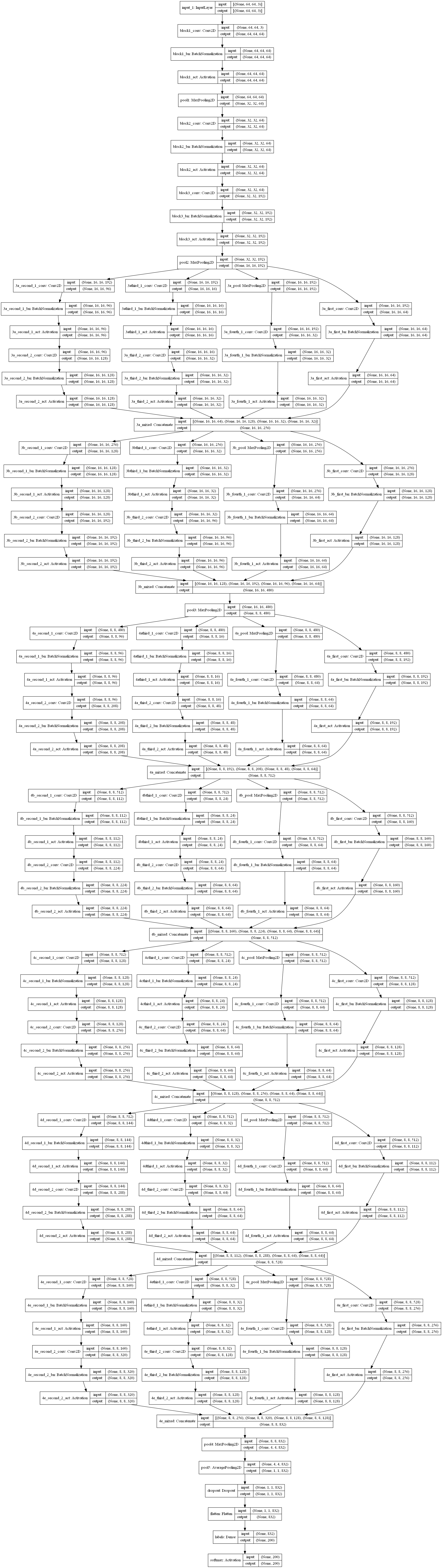

It has been a while I didn't update the "small task list" in this repo. This time I explore methods to use open image dataset v4, obtain the annotations for any class that I want to detect, and finally created a detector that only detect human face (instead of the 80 classes of objects in yolo by default).


As it is horribly frustrating to understand code merely by watching, I have devided the code into several blocks, added numerical examples and explain the shape of the variables to make yolov3 code base more easy to digest.
This time we create a simple poetry generator. We create an encoder (a model) that is then trained by a set of sentences of list of poems and by using the pretrained weight of glove embedding word vectors (50-dimensional).
Upon model.fit, we reuse the same lstm layer to create another model (called sample_model) that can repeatedly geneate next word based on the current word, which takes the form:
[[text], [hidden state], [cell state]] |-> [[text], [hidden state], [cell state]].