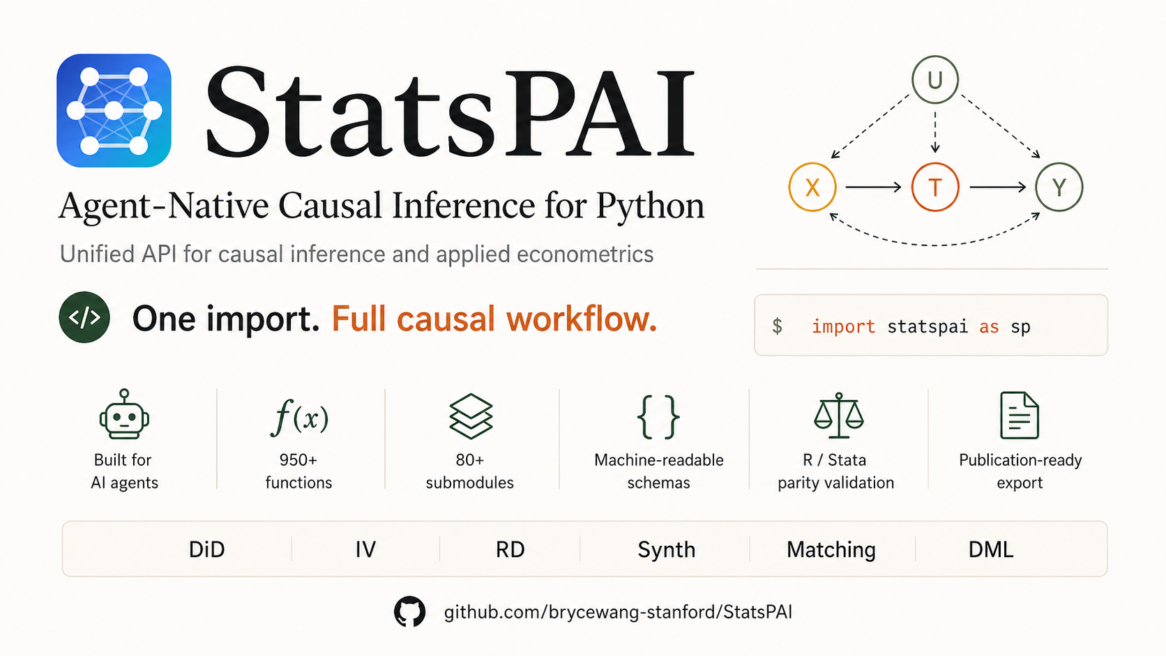








StatsPAI is for empirical researchers who would normally jump between Stata, R, and Python. Its goal is to make common Stata/R econometrics and causal-inference workflows feel native in Python: load a dataset, estimate a model, inspect diagnostics, export tables, and hand the result to an agent or notebook without leaving one API.
It is meant to be a practical replacement path for new Python-first work:
- Stata-style routines:
regress,ivregress,reghdfe,csdid,rdrobust,synth,psmatch2,outreg2. - R-style routines:
lm,fixest,did,rdrobust,Synth,DoubleML,MatchIt,modelsummary,broom. - Python-native outputs:
.summary(),.tidy(),.plot(),.to_latex(),.to_docx(),.to_agent_summary()where supported by the result object. - Companion Stata tooling: our own
stata-codecan work with StatsPAI so agents can understand existing Stata workflows, translate them into Python, and cross-check results more smoothly. - Companion skill repos:
Auto-Empirical-Research-Skills,AER-Skills,Awesome-Journal-Skills, andPaper-WorkFlowcan work alongside StatsPAI and an agent as the methods, journal, manuscript, and reproducibility skill layer.
StatsPAI is not a promise that every Stata/R command is bit-for-bit identical.
When exact external parity matters, use the validation_status metadata,
the reference-parity tests, and sp.cross_validate to see what has been
certified for that estimator.
pip install statspaiThen:
import statspai as sp

print(sp.datasets.list_datasets()[["name", "design", "n_obs"]].head())
StatsPAI ships teaching datasets such as Card (1995), Callaway-Sant'Anna
mpdta, Lee (2008) RD, LaLonde/NSW, and California Proposition 99. The examples
below run offline after installation.
At a glance: 1,139 registered functions across 87 submodules; 339k LOC (core) + 182k LOC (tests). Run python scripts/registry_stats.py to reproduce these numbers.
| What you used before | Stata / R examples | StatsPAI entry point |
|---|---|---|
| OLS / robust SE | reg y x, vce(robust) / lm() + sandwich |
sp.regress(..., robust="hc1") |
| IV / 2SLS | ivregress 2sls / AER::ivreg() |
sp.ivreg("y ~ (d ~ z) + x", data=df) |
| High-dimensional FE | reghdfe / fixest::feols() |
`sp.feols("y ~ x |
| Staggered DiD | csdid / did::att_gt() |
sp.callaway_santanna() + sp.aggte() |
| Regression discontinuity | rdrobust / rdrobust::rdrobust() |
sp.rdrobust() |
| Synthetic control | synth / Synth::synth() |
sp.synth() |
| Matching / PSM | psmatch2 / MatchIt |
sp.psmatch2() and matching helpers |
| Publication tables | outreg2, esttab / modelsummary |
sp.outreg2(), sp.modelsummary() |
StatsPAI is meant to be the broad Stata/R-style workbench for applied empirical research, not only a single modeling family.
| Package | Best fit | Where StatsPAI is different |
|---|---|---|
causallib |
Observational causal inference with a scikit-learn-style workflow: IPW, matching, standardization, doubly robust estimation, and evaluation. | StatsPAI is broader for Stata/R migration: OLS, IV, high-dimensional FE, DiD, RD, synthetic control, matching, diagnostics, validation metadata, and publication-table export in one API. |
CausalPy |
Bayesian causal analysis for quasi-experimental settings, built around PyMC models, uncertainty, and visual diagnostics. | StatsPAI prioritizes familiar Stata/R econometrics commands, frequentist workflows, cross-language parity evidence, bundled teaching datasets, and agent-ready result summaries. |
Use causallib when you mainly want sklearn-style treatment-effect pipelines.
Use CausalPy when you want Bayesian causal modeling in PyMC. Use StatsPAI when
you want one Python package to replace the everyday Stata/R empirical workflow.
The outputs below are rounded from the bundled examples in this repository using StatsPAI 1.20.0.
Question: how much higher is log wage for one more year of schooling in the Card (1995) teaching dataset?
import statspai as sp

card = sp.datasets.card_1995()
ols = sp.regress(
    "lwage ~ educ + exper + expersq + black + south + smsa",
    data=card,
    robust="hc1",
)
print(ols.summary())
Result:
Model: OLS
Dependent Variable: lwage

              Coefficient  Std. Error  t-statistic  P>|t|
Intercept          4.8388      0.0637      76.0131 0.0000
educ               0.1100      0.0041      26.5543 0.0000
exper              0.0283      0.0054       5.2742 0.0000
expersq           -0.0005      0.0002      -2.2132 0.0270
black             -0.1561      0.0231      -6.7571 0.0000
south             -0.0554      0.0193      -2.8636 0.0042
smsa               0.0905      0.0205       4.4214 0.0000

R-squared: 0.2307
Read it like a Stata/R regression table: in this replica, one additional year
of schooling is associated with about 0.110 higher log wage, before dealing
with endogeneity. Adding the standard Card (1995) controls (experience and
its square, race, region, SMSA) lifts R² from 0.210 to 0.231 and the
educ coefficient is essentially unchanged — the small attenuation from
classical measurement error in educ persists and motivates the IV in
example 2.
Question: instrument education with proximity to a four-year college (nearc4).
import statspai as sp

card = sp.datasets.card_1995()
iv = sp.ivreg(
    "lwage ~ (educ ~ nearc4) + exper + expersq + black + south + smsa",
    data=card,
)
print(iv.summary())
Result:
Model: IV-2SLS
Dependent Variable: lwage

           Coefficient  Std. Error  t-statistic  P>|t|
educ            0.1418      0.0188       7.5606 0.0000

Model Diagnostics:
First-stage F (educ): 159.8305
Partial R2 (educ)   : 0.0505
Hausman p-value     : 0.0322
StatsPAI prints the coefficient and the diagnostics you would usually collect with separate post-estimation calls.
Question: what is the average minimum-wage effect on teen employment in the
Callaway-Sant'Anna mpdta example?
import statspai as sp

mp = sp.datasets.mpdta()
gt = sp.callaway_santanna(
    data=mp,
    y="lemp",
    t="year",
    i="countyreal",
    g="first_treat",
)
overall = sp.aggte(gt, type="simple", bstrap=False)
print(overall.summary())
Result:
Callaway and Sant'Anna (2021) - aggte[simple]

ATT:        -0.032977
Std. Error:  0.005493
95% CI:     [-0.043742, -0.022211]
P-value:     0.0000
Observations: 2,500
The headline estimate is negative and statistically precise in this bundled replica.
Question: is there an incumbent advantage at the zero-margin cutoff in the Lee (2008) Senate election design?
import statspai as sp

lee = sp.datasets.lee_2008_senate()
rd = sp.rdrobust(data=lee, y="voteshare_next", x="margin", c=0)
print(rd.summary())
Result:
Sharp RD Estimation

RD Effect:   0.061599
Std. Error:  0.022662
95% CI:     [0.017183, 0.106015]
P-value:     0.0066

Bandwidth H: 0.042287
N Effective Left: 440
N Effective Right: 443
The robust bias-corrected RD estimate is about 0.062 vote-share points.
Question: how did California's Proposition 99 affect cigarette sales?
import statspai as sp

prop99 = sp.datasets.california_prop99()
sc = sp.synth(
    data=prop99,
    outcome="cigsale",
    unit="state",
    time="year",
    treated_unit="California",
    treatment_time=1989,
)
print(sc.summary())
Result:
Synthetic Control Method

ATT:        -13.085166
Std. Error:  4.164718
95% CI:     [-21.247862, -4.922469]
P-value:     0.0789

Active donor weights:
Montana  0.8420
Nevada   0.1580
The estimate says California consumed about 13 fewer packs per capita after the intervention in this replica.
Every result object ships with Stata-style and R (modelsummary/broom)
exporters. One call drops a multi-sheet .xlsx or a Word table that you can
hand to a co-author.
sp.outreg2(r1, r2, filename="results.xlsx")            # Excel, Stata-style
sp.modelsummary(r1, r2, output="table.docx")            # Word, modelsummary-style
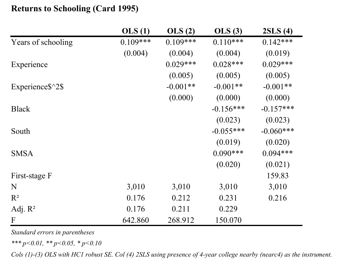
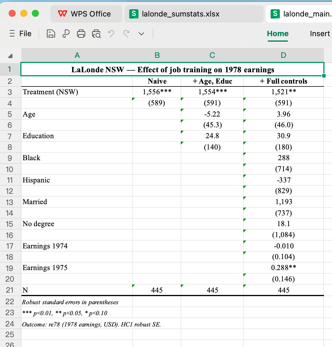
The screenshots above are the .xlsx output of sp.outreg2 on the Card (1995)
OLS + IV pair and the LaLonde/NSW propensity-score regression. Each sheet
contains the coefficient table, model-fit statistics, and significance stars
in the format your journal template expects.
If you miss Stata's Graph Editor, use sp.interactive(fig) on any matplotlib
figure returned by StatsPAI. It opens a Jupyter editing panel with a live
preview, so beginners can adjust a figure without learning every matplotlib
option first.
What it is for:
- change titles, labels, fonts, colors, markers, line widths, grids, legends, axis limits, figure size, and export DPI;
- switch among publication-oriented themes, including academic, ggplot-like, FiveThirtyEight-style, and dark presentation styles;
- keep the data layer protected while editing cosmetic elements;
- export reproducible Python code for the edits, so the final figure can be regenerated from a script instead of being only a manual screenshot.
import statspai as sp

mp = sp.datasets.mpdta()
gt = sp.callaway_santanna(data=mp, y="lemp", t="year",
                          i="countyreal", g="first_treat")
agg = sp.aggte(gt, type="dynamic", bstrap=False)
fig, ax = sp.ggdid(agg)

editor = sp.interactive(fig)   # edit the plot in Jupyter
print(editor.generate_code())  # copy reproducible matplotlib edits
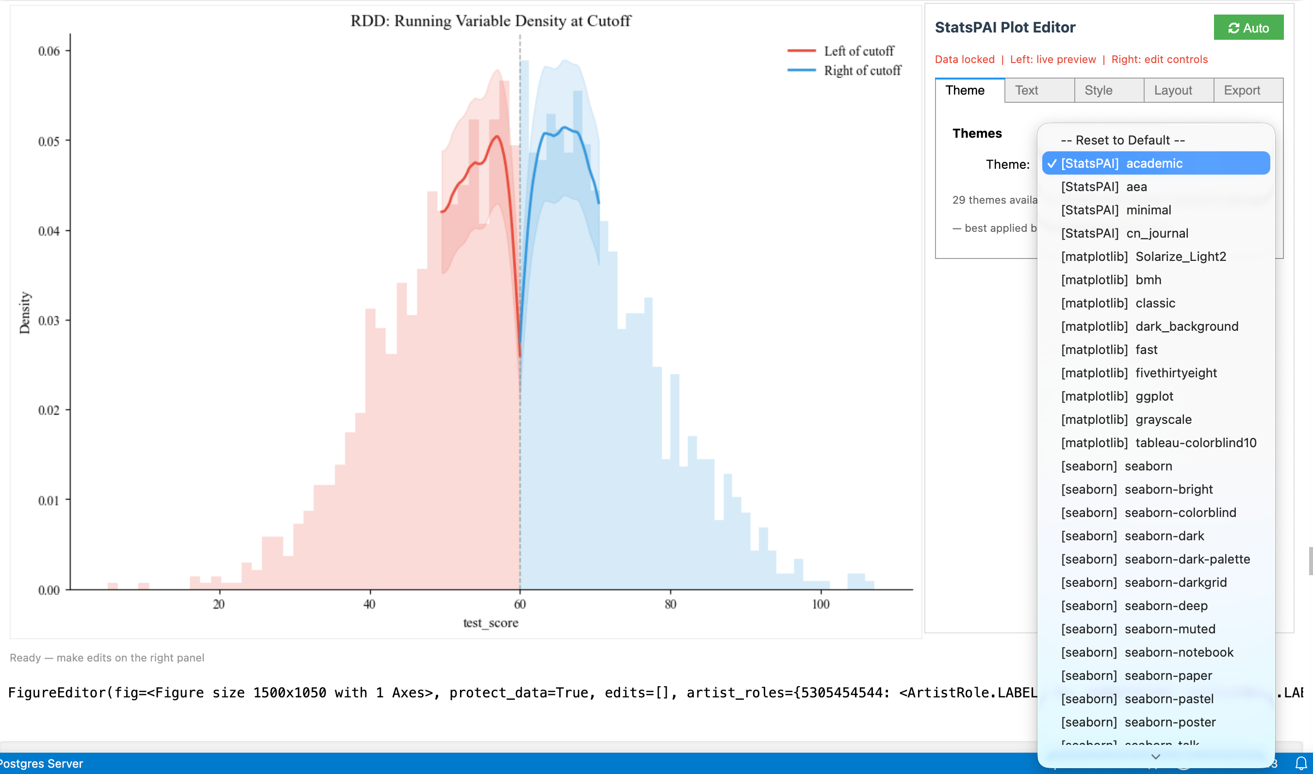
The screenshot above shows the intended workflow: preview on one side, editing controls on the other, and code export for reproducibility.
import statspai as sp

card = sp.datasets.card_1995()
r1 = sp.regress(
    "lwage ~ educ + exper + expersq + black + south + smsa",
    data=card,
    robust="hc1",
)
r2 = sp.ivreg("lwage ~ (educ ~ nearc4) + exper + expersq + black + south + smsa", data=card)

print(r1.summary())                         # human-readable table
print(r1.tidy().head())                      # broom-style dataframe
sp.modelsummary(r1, r2, output="table.docx") # Word table
sp.outreg2(r1, r2, filename="results.xlsx")  # Stata-style export
Useful docs:
- Getting started
- Cookbook
- Choosing an IV estimator
- Choosing a DID estimator
- Choosing an RD estimator
- Migrating from R to StatsPAI
- Exporting regression tables
StatsPAI has a large API surface, so validation status matters.
import statspai as sp

print(sp.describe_function("ivreg")["validation_status"])
print(sp.list_functions(validation_status="certified")[:5])
Use the validation metadata to distinguish:
- certified functions with external numerical evidence;
- validated functions with internal or published-reference checks;
- API-stable functions whose interface is stable but whose exact Stata/R parity may be design-dependent;
- experimental functions for frontier workflows.
Agent-facing metadata is available through sp.list_functions(),
sp.describe_function(), and sp.function_schema().
The validation tier above has a richer, auditable backing: a parity index
where every verified function records what it was aligned against, to what
tolerance, on which test, and how closely it matched. Each row traces to a
committed test artifact (the pinned StatsPAI ↔ R ↔ Stata harness, version-locked
via renv.lock + per-run provenance) — nothing is asserted from memory.
import statspai as sp

sp.parity_status("feols")
# {'status': 'bit-exact', 'reference': 'fixest::feols',
#  'reference_versions': {'R': '...4.5.2...', 'fixest': '0.14.0'},
#  'tolerance': 'rel_est<=1e-06, rel_se<=1e-06', 'headline': {...}, 'test': [...]}

sp.parity_summary()              # honest coverage counts (verified vs unverified)
sp.parity_matrix(status="bit-exact")
Grades: bit-exact (machine tolerance vs a named R/Stata reference), aligned
(documented looser tolerance), analytical-only (recovers a known DGP truth),
external-replication (published-paper numbers), and unverified (registered
but no parity evidence attached yet — the honest gap). The full,
auto-generated matrix is published at
docs/parity.md.
Release notes live outside the README:
- CHANGELOG.md for the full version history.
- Docs changelog page for the rendered documentation site.
The README is intentionally focused on first-time users.
StatsPAI is under JOSS review. Reviewers can start with:
If you use StatsPAI in research, cite the package and the underlying method
papers for each estimator. sp.citation() returns the package citation, and
many result objects expose estimator-level citation helpers.
@software{wang2026statspai,
  author  = {Wang, Biaoyue and Rozelle, Scott},
  title   = {StatsPAI: Validation-Tiered Causal Inference and
             Econometrics Workflows for Python},
  year    = {2026},
  version = {1.20.0},
  url     = {https://github.com/brycewang-stanford/StatsPAI}
}MIT. See LICENSE.