This project contains methods to solve the forward problem of Magneto Acousto Electric Tomography (MAET).

MAET is a medical imaging modality, which recovers the conductivity of tissue. A MAET image is obtained by placing the tissue of interest in a conductive medium, and coupling planar acoustic waves with a constant magnetic field to generate electrical signals. Let $M(t)$ denote our measurement at time $t$. If we are using a pair of electrodes at points $z_1, z_2$ on the boundary of the apparatus, our measurements are given by $M(t) = u(t,z_1)-u(t,z_2)$, where $u(t,x)$ denotes the electric potential of the tissue.

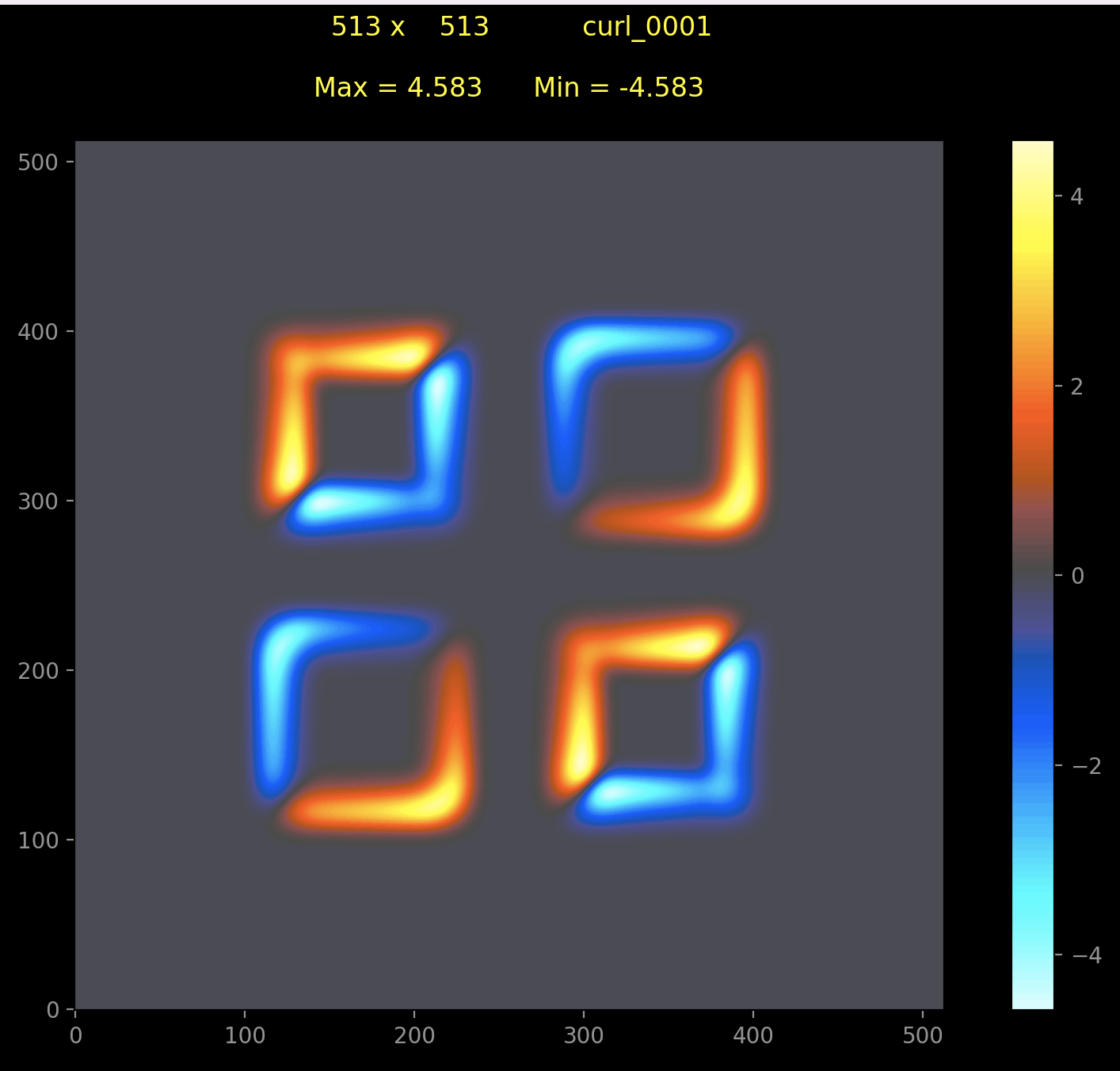
Let $J$ denote the "lead" current that would flow through the tissue if a unit current were injected at the point $z_1$ and extracted at the point $z_2$. It can be shown that $M(t) = \frac{B}{\rho}\cdot \left( R(\nabla \times J(x)) \right)$, where $R$ denotes the Radon transform, $B$ is the magnetic field, and $\rho$ is the density of the tissue, assumed to be constant. Thus, the measurements of differences on electric potential are proportional to the curl of lead current.

The primary purpose of this project is to simulate lead currents for the testing of MAET inversion procedures.

Suppose we inject currents at a finite set of points $W_j$, with $\sum W_j= 0$ over a region of constant conductivity $\sigma_0$. The resulting electric potential is given by $w(x) = -\frac{1}{\sigma_0}\sum W_j\phi(x-y^{(j)})$, where $\phi(x)=\frac{1}{2\pi}\ln|x|$ is the fundamental solution to Laplace's Equation. Consider now a simply connected region $\Omega$ not containing any of the injection points where conductivity is non-constatnt. The equation governing the resulting electric potential over $\Omega$ is given by $\nabla \cdot \sigma(x) (u(x)+w(x)) = 0, \quad x\in \mathbb{R}^2\setminus \cup_{j=1}^{n}y^{(j)}, \quad \lim_{|x|\rightarrow \infty}u(x)=0$. This is the conductivity equation.

Let $U(x) = \Delta u(x)$. We can express the conductivity equation as a Fredholm equation of the second kind: $U(x)+ \left[ \frac{\partial \ln \sigma(x)}{\partial x_1}\int_{\Omega}\phi(x-y)\frac{\partial}{\partial y_1}U(y)dy + \frac{\partial \ln \sigma(x)}{\partial x_2}\int_{\Omega}\phi(x-y)\frac{\partial}{\partial y_2}U(y)dy \right] = -\nabla \ln \sigma(x) \cdot \nabla w(x)$.

Given an initial configuration of point sources and an initial conductivity function, we compute $U(x)$ via GMRES, and invert the laplacian with a Sine Series to obtain the electric potential, $u(x)$. From $u(x)$, we can use standard methods to compute electrical currents and their curls. Note that special care must be taken to handle the singular kernels in the above convolutions. A method is outlined in the results folder which explains how to compute those convolutions.

The main script to be run is "currents.py" which is located in src/scripts/. The supporting functions are defined in the modules in the "main" folder. This script will output .d files for the curl, currents, error, conductivity, and electric potential, as well as drawings of the current lines. The method simulates an experiment where the tissue is rotated in a chamber, and executes as many rotations as specified in the "currents.cfg" file. "currents.cfg" also contains parameters to determine the configuration of point sources, and the form of the conductivity function.

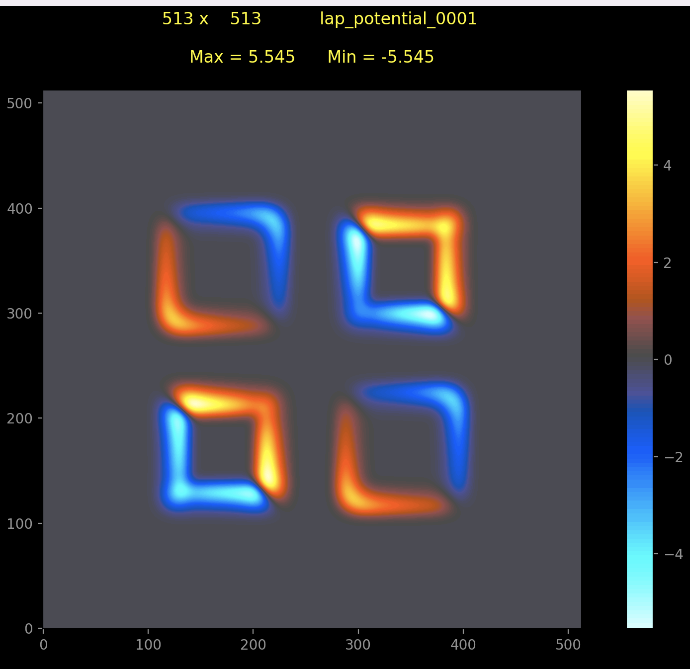
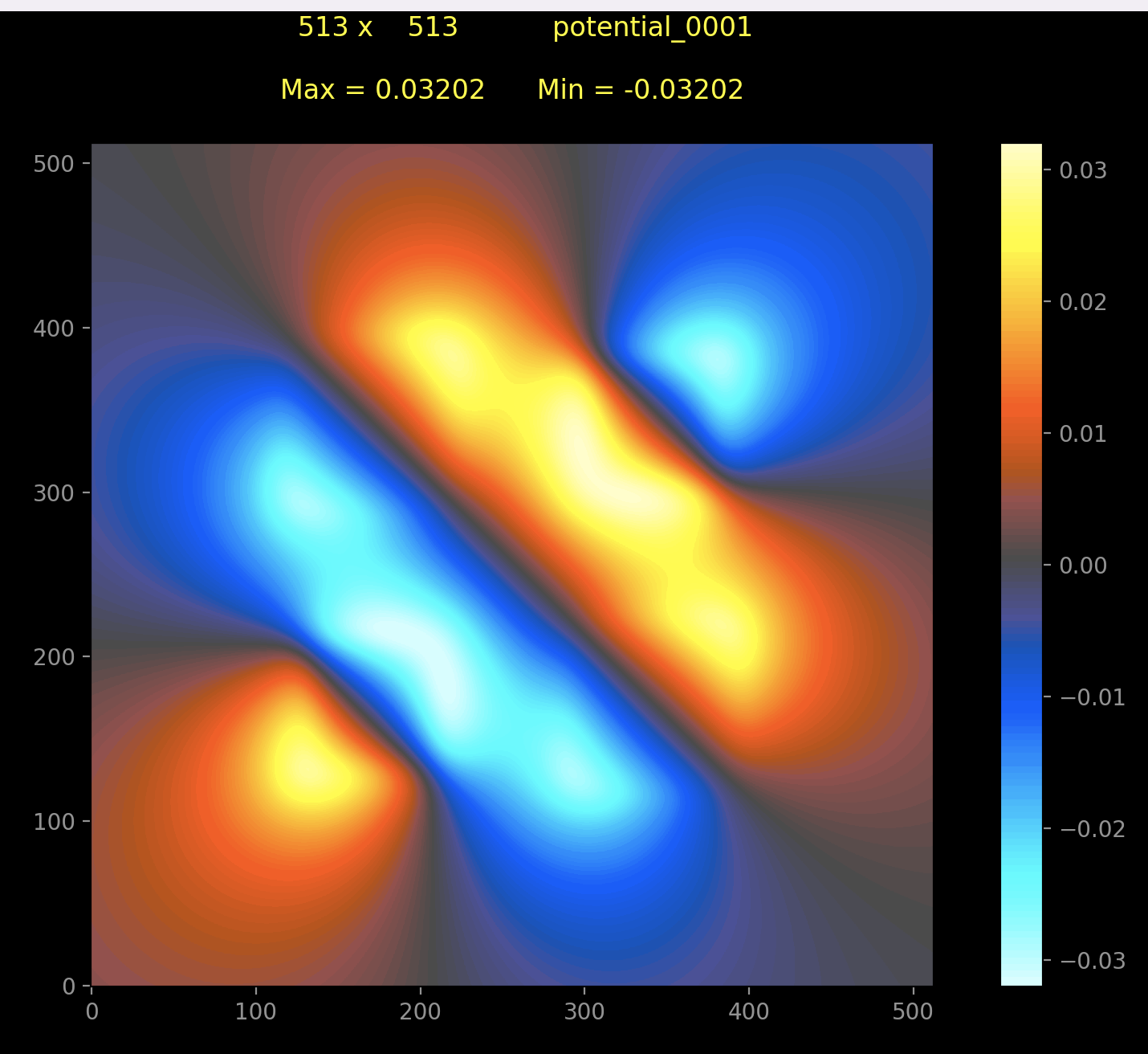
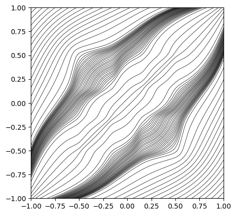
The below figures are examples of the Laplacian of Potential, the Potential, the Current Lines, and the Curl of Current.

References

[1] Kunyansky, Leonid. "A Mathematical Model and Inversion Procedure for Magneto-acousto-electric Tomography." Inverse Problems 28.3 (2012): 35002-21. Web.