The honest, code-checked support matrix for Vinculum. Every claim here
is verified against MathSymbolTable.swift, MathParser.swift, the
Layout+*.swift builders, and the golden fixtures in
Tests/fixtures/math-golden/. The figures are CI-regenerated from the live
engine on every push to main — if a figure looks wrong, the engine is
wrong, and that has already caught real bugs (a mis-seated \vec arrow,
dots dropped from the symbol charts).
How degradation works. Vinculum never throws and never half-renders. An
unknown command becomes an .unsupported leaf; MathParser.isFullySupported
returns false for any tree that contains one; and MathImageRenderer returns
nil so the host shows its own fallback.
MathParser.unsupportedCommands(in:limit:) names the offending commands so a
fallback card can say why. MathParser.parse is total — the worst case is a
single .unsupported(source) leaf, never a crash.
Legend: ✅ native render ·
Scale (verified counts): 404 symbol-table commands (symbolTable) +
37 function-name operators (functionNames) — roughly ~400 commands in
total, across every TeX atom class, each carrying its correct inter-atom
spacing class.
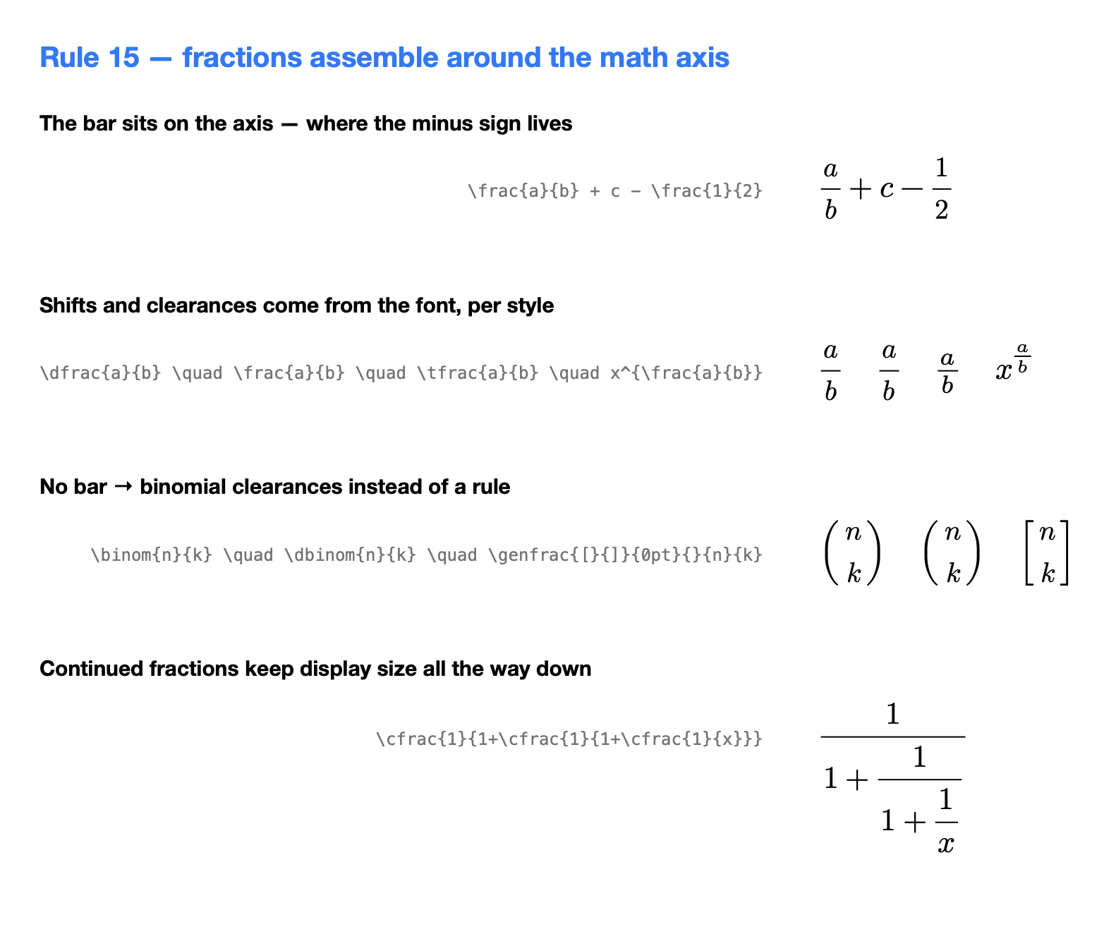
| Command | Status | Example | Note |
|---|---|---|---|
\frac |
✅ | \frac{a}{b} |
Ruled, axis-aligned |
\cfrac |
✅ | \cfrac{1}{1+\cfrac{1}{x}} |
Full-size continued fraction; optional [l]/[r] numerator alignment (amsmath default centered) |
\binom |
✅ | \binom{n}{k} |
Ruleless, paren-fenced |
\dfrac / \tfrac |
✅ | \dfrac{a}{b} |
Force display / text style regardless of ambient context |
\dbinom / \tbinom |
✅ | \dbinom{n}{k} |
Force display / text style |
\genfrac |
✅ | \genfrac{[}{]}{0pt}{}{n}{k} |
Custom left/right delims, rule on/off (0pt → no rule), forced style (0=display, 1/2/3=text) |
\over \atop \choose \brace \brack |
✅ | {n \brace k} |
TeX infix forms: numerator = everything before, denominator = everything after, in the group |
\frac{-b \pm \sqrt{b^2 - 4ac}}{2a} \qquad \cfrac{1}{1 + \cfrac{1}{1 + \cfrac{1}{x}}}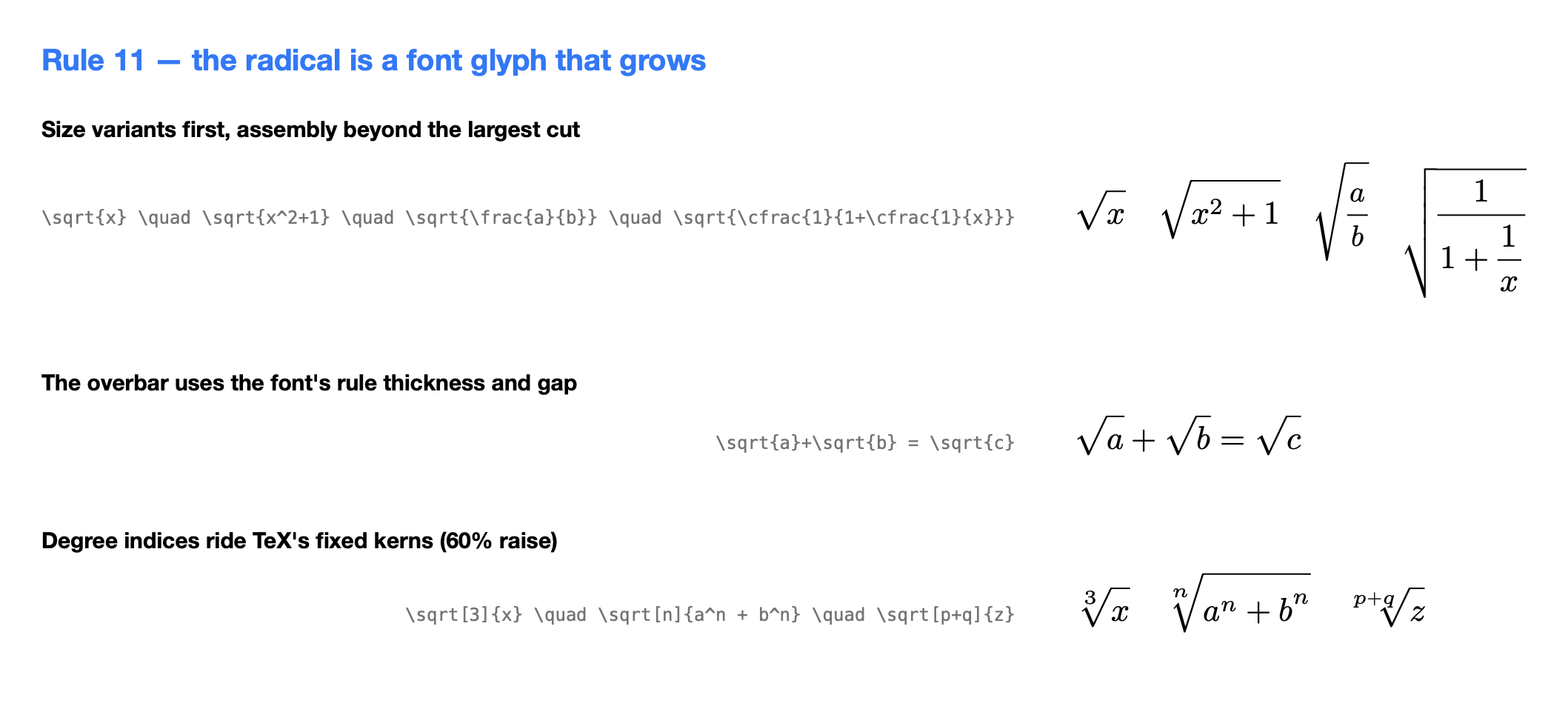
| Command | Status | Example |
|---|---|---|
\sqrt |
✅ | \sqrt{2} |
\sqrt[n]{} |
✅ | \sqrt[3]{x^2 + y^2} |
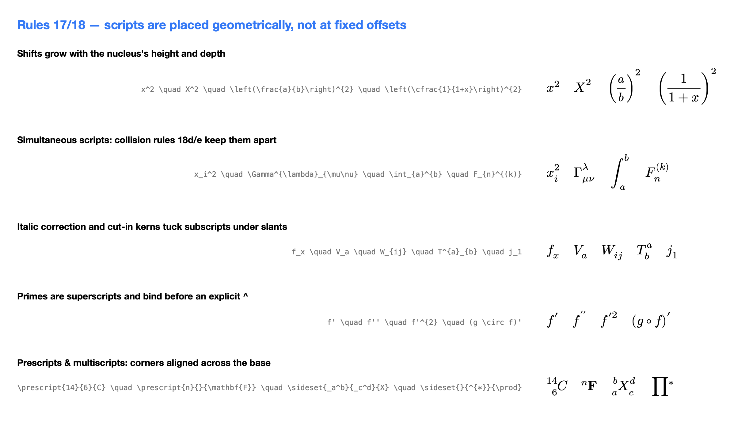
| Feature | Status | Example |
|---|---|---|
| Superscript | ✅ | x^2 |
| Subscript | ✅ | x_i |
| Both | ✅ | a_{i,j}^{(k)} |
| Nested | ✅ | x^{2^{n}} |
| Stacked limits (display) | ✅ | \sum_{i=1}^{n} — symbol operators stack in display |
| Primes as raised glyphs | ✅ | f', f'' render as raised, coalesced primes (′); f'^2 merges the primes then the exponent |
| Prescripts | ✅ | \prescript{n}{m}{X} — mathtools left scripts (isotopes ¹⁴₆C, tensors) |
| Multiscripts | ✅ | \sideset{_a^b}{_c^d}{X} — scripts at all four corners; the base keeps its own limits |
Cramped style (denominators, radicands) lowers superscripts per TeX. Pre- and post-scripts share one pair of baseline shifts so every corner aligns across the base; the post-superscript rides the italic correction, the pre-scripts hug the base's left edge.
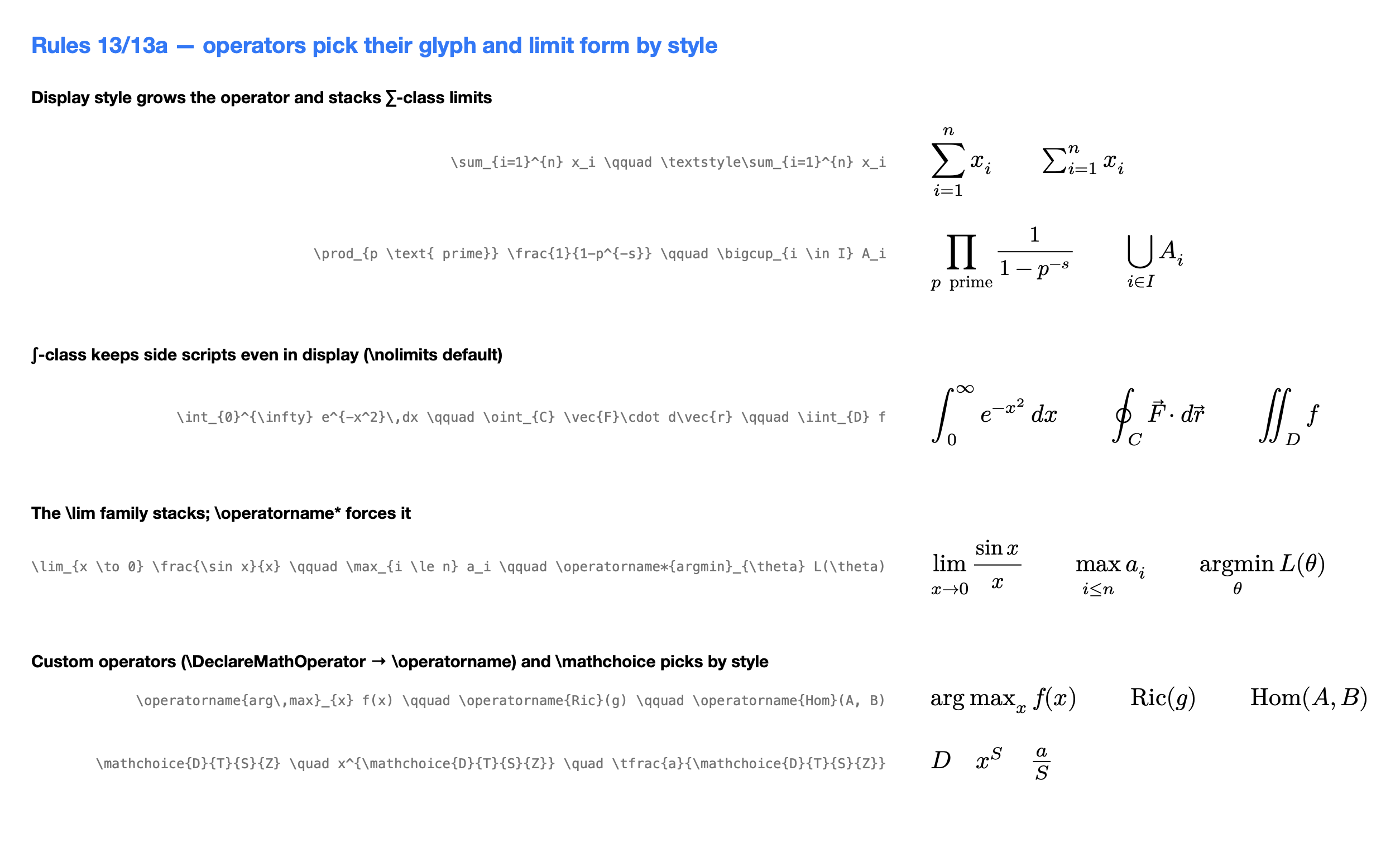
Operators whose limits stack above/below in display style and sit as scripts inline:
\sum  \prod  \bigcup  \bigcap  \coprod  \biguplus  \bigsqcup
\bigvee  \bigwedge  \bigoplus  \bigotimes  \bigodot
Integral-class operators correctly keep their scripts to the side even in
display — TeX's default for that class (the same placement \nolimits forces
explicitly for ∑-class operators):
\int \iint \iiint \iiiint \oint \oiint \oiiintNamed function operators that stack their limit underneath in display style
(\lim_{x\to0}), matching TeX: \lim \max \min \sup \inf \det \gcd \Pr \deg \dim \ker \hom \arg \limsup \liminf \argmin \argmax. All other function names
(\sin \cos \log \ln …) render upright with side scripts. \mathop{…} and
\operatorname*{…} also stack (see below).
All carry correct TeX atom classes, so inter-atom spacing is real.
- Greek — lowercase
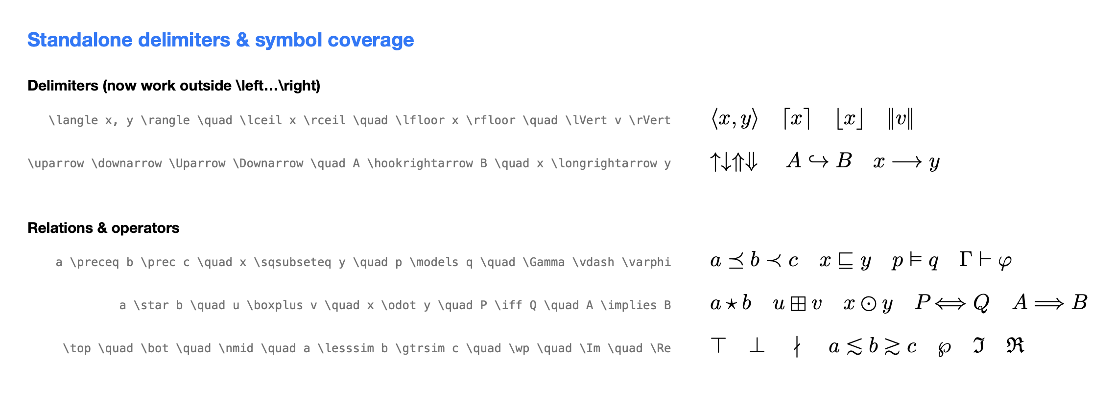
\alpha…\omegaplus variants (\varepsilon \vartheta \varpi \varsigma \varphi \varkappa \varrho \digamma), uppercase\Gamma…\Omega. - Binary operators —
\pm \mp \times \div \cdot \ast \cup \cap \setminus \oplus \otimes \wedge \vee \circ \star \bullet \dagger \ddagger \sqcup \sqcap \uplus \odot \ominus \oslash \boxplus \boxtimes \triangleleft \triangleright \diamond \bigtriangleup \bigtriangledown \ltimes \rtimes \barwedge \veebar \boxdot \boxminus \circledast \dotplus \intercal \smallsetminus \Cap \Cup … - Relations —
\leq \geq \neq \equiv \approx \sim \simeq \cong \propto \subset \supset \subseteq \supseteq \in \ni \notin \prec \succ \preceq \succeq \models \vdash \dashv \asymp \doteq \sqsubseteq \gtrsim \lesssim \ll \gg \perp \parallel \mid \nmid \leqslant \geqslant \leqq \geqq \lll \ggg \vDash \Vdash \multimap …, negated relations\nleq \ngeq \nless \nsim \ncong \nsubseteq \nvdash \lneq \subsetneq …, and arrows\to \rightarrow \leftarrow \Rightarrow \Leftrightarrow \mapsto \hookrightarrow \longrightarrow \iff \implies \uparrow \twoheadrightarrow \rightarrowtail \curvearrowright \leftrightarrows \Rrightarrow \longmapsto \nrightarrow …plus harpoons (\leftharpoonup \rightharpoondown \leftrightharpoons …). - Ordinary —
\infty \partial \nabla \forall \exists \nexists \emptyset \varnothing \hbar \hslash \ell \Re \Im \aleph \beth \gimel \daleth \angle \measuredangle \sphericalangle \neg \top \bot \flat \sharp \natural \clubsuit \heartsuit \wp \complement \square \blacksquare \checkmark \lozenge \blacktriangle \imath \jmath \Bbbk \eth …. - Ellipses —
\dots \ldots \cdots \ddots \dotsb \dotsc \dotsm \dotsi \dotsoare Inner atoms (plain TeX defines them as\mathinner), so they draw thin spaces on both sides —f(x_1,\ldots,x_n)spaces the way the TeXbook sets it.\vdotsis ordinary. - Standalone delimiters (usable outside
\left…\right):\langle \rangle \lceil \rceil \lfloor \rfloor \lbrace \rbrace \lbrack \rbrack \lvert \rvert \lVert \rVert \vert \Vert \backslash. - Escaped literals —
\{ \} \| \$ \% \& \#. - Direct Unicode — typing
∫ ∑ ≤ α →directly gets the same atom class its command spelling would, so spacing and operator limits still work.
For the exhaustive command-by-command index — with a rendered specimen
chart per atom class — see COMMANDS.md; for the raw set see
MathSymbolTable.swift (symbolTable, 404 entries) and the functionNames
set (37 entries).
Force the inter-atom spacing class of a subexpression:
| Command | Forces class | Note |
|---|---|---|
\mathbin |
binary | a \mathbin{\star} b |
\mathrel |
relation | |
\mathop |
large operator | Also takes stacked display limits (\mathop{\oplus}\limits_{i}) |
\mathord |
ordinary | |
\mathinner |
inner | Thin-spaced subformula (what fractions and \left…\right get automatically) |
\mathopen |
opening | |
\mathclose |
closing | |
\mathpunct |
punctuation |
All ✅.
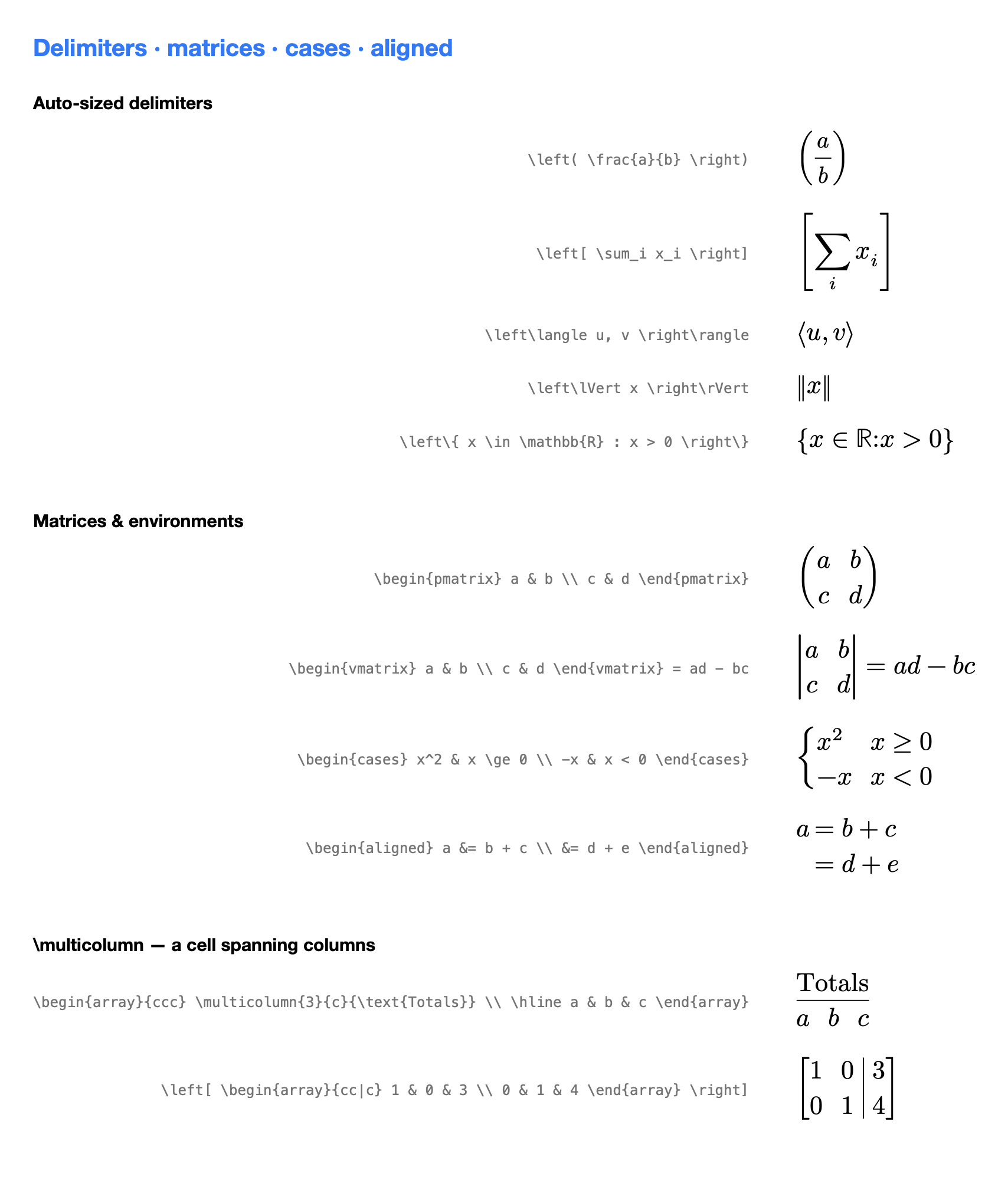
| Environment | Status | Fences / alignment |
|---|---|---|
matrix |
✅ | none, centered |
pmatrix |
✅ | ( ) |
bmatrix |
✅ | [ ] |
Bmatrix |
✅ | { } |
vmatrix |
✅ | | | |
Vmatrix |
✅ | ‖ ‖ |
smallmatrix |
✅ | script-size grid, no fences |
cases |
✅ | {, left-aligned columns |
aligned / align / alignat / alignedat / split / gather / gathered / multline |
✅ | alignment at & |
substack |
✅ | tight centered stack (script size) |
array |
✅ | {l c r | c} per-column alignment + | vertical rules + \hline / \cline{i-j} — augmented matrices [A|b], bordered/truth tables |
\multicolumn{n}{align}{…} |
✅ | A cell spanning n columns with its own l/c/r alignment; overflow grows the span. Works in every grid environment |
arraydraws\hline/\cline{a-b}and|column rules. In the other environments those tokens are consumed and ignored (they don't flip the grid to a fallback).alignat{n}/alignedat{n}: the{n}column count is consumed correctly (it used to leak into the first cell).- Starred forms
align*,pmatrix*,matrix*etc. are accepted. A trailing column-alignment bracket (pmatrix*[r],matrix*[l]) applies its alignment uniformly to every column.
\begin{pmatrix} a & b \\ c & d \end{pmatrix}
\begin{cases} x^2 & x \ge 0 \\ -x & x < 0 \end{cases}
\begin{aligned} a &= b + c \\ &= d + e \end{aligned}
\begin{array}{c|c} A & b \\ \hline 1 & 2 \end{array}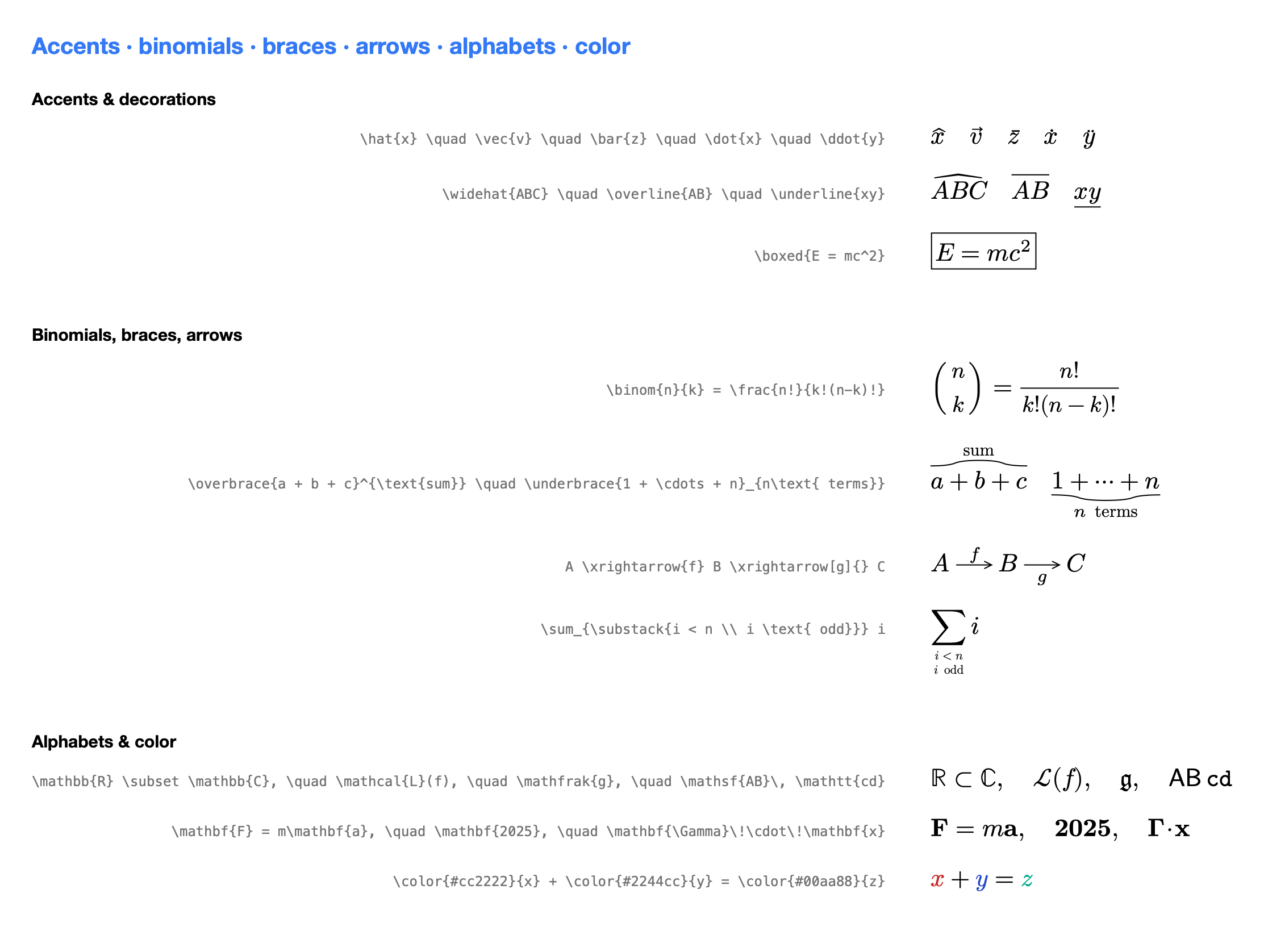
Mapped to Unicode Mathematical Alphanumeric Symbols; CoreText resolves them through STIX Two / Apple Symbols (no bundled font needed). The pre-Unicode "Letterlike Symbols" holes (ℝ ℂ ℋ ℯ …) are handled by exception tables.
| Command | Alphabet | Digits? | Notes |
|---|---|---|---|
\mathbb |
blackboard 𝔸 | ✅ | Holes: ℂ ℍ ℕ ℙ ℚ ℝ ℤ |
\mathcal / \mathscr |
script 𝒜 | ❌ | Holes: ℬ ℰ ℱ ℋ ℐ ℒ ℳ ℛ ℯ ℊ ℴ |
\mathfrak |
fraktur 𝔞 | ❌ | Holes: ℭ ℌ ℑ ℜ ℨ |
\mathsf |
sans-serif 𝖠 | ✅ | |
\mathtt |
monospace 𝙰 | ✅ | |
\mathbf |
bold 𝐀 | ✅ | Codepoint-mapped: bold letters 𝐀…𝐳, bold Greek 𝚨…𝛚, bold digits 𝟎…𝟗 |
\boldsymbol / \bm |
bold-italic 𝑨 | bold digits | Codepoint-mapped |
\pmb |
≈ bold | — | "Poor-man bold" approximated as \mathbf |
\mathbb{R} \subset \mathbb{C}, \quad \mathcal{L}(f), \quad \mathfrak{g}, \quad \mathsf{AB}\,\mathtt{cd}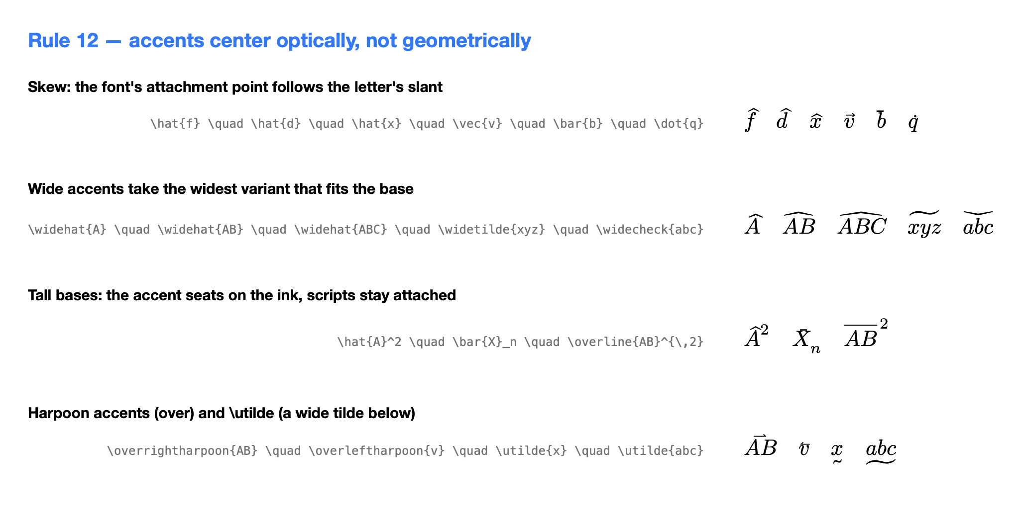
| Kind | Commands | Status |
|---|---|---|
| Point accents | \hat \check \tilde \bar \vec \dot \ddot \breve \mathring \acute \grave |
✅ |
| Stretchy | \widehat \widetilde \widecheck |
✅ (walk the font's horizontal width-variant ladder; widest drawn cut that fits) |
| Harpoon (over) | \overrightharpoon \overleftharpoon |
✅ (stretchy, tracks the base width) |
| Under-accent | \utilde |
✅ (a wide tilde below the base, stretchy) |
| Rules | \overline \underline |
✅ (drawn rule, not a glyph) |
Point accents use ink extents (not the loose typographic box) for
placement, with the skew coming from each glyph's topAccentAttachment —
that's why \hat{f} leans with the f. \vec (the one accent whose only
spelling is a combining mark) routes through the font's glyph-ID path so its
arrow seats exactly on the letter.
\hat{x} \quad \vec{v} \quad \bar{z} \quad \widehat{ABC} \quad \widecheck{f} \quad \overline{AB}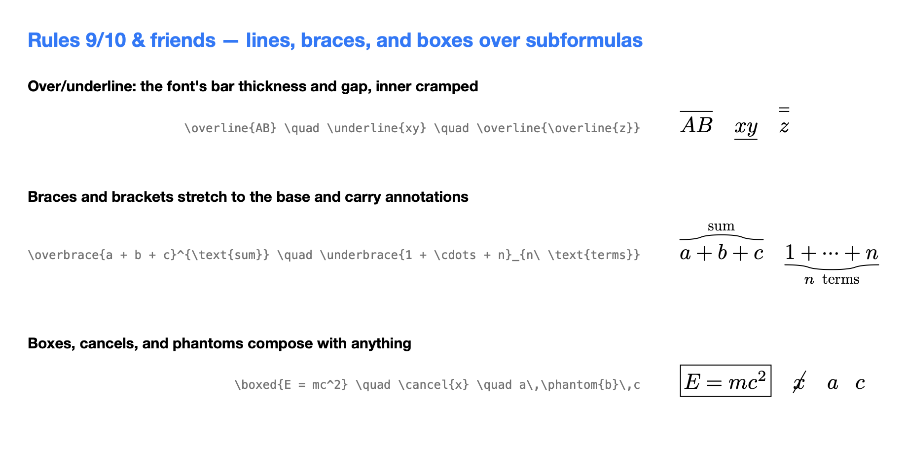
| Command | Status | Example |
|---|---|---|
\overset / \underset / \stackrel |
✅ | \stackrel{?}{=} |
\overbrace{}^{label} |
✅ | \overbrace{a+b+c}^{\text{sum}} |
\underbrace{}_{label} |
✅ | \underbrace{1+\cdots+n}_{n\text{ terms}} |
\overbracket / \underbracket |
✅ | Square-bracket brace with vertical end tines |
\overparen / \underparen |
✅ | Parenthesis-style arc |
\overrightarrow / \overleftarrow / \overleftrightarrow |
✅ | Vector arrows over the content: \overrightarrow{AB} |
\underrightarrow / \underleftarrow / \underleftrightarrow |
✅ | Arrows drawn under the content |
Braces/brackets/parens are drawn as hand-stroked paths; arrows are a stretchy shaft plus a drawn head sized to fit the label.
\x…arrow[under]{over}: an arrow that stretches to the wider of its optional
[under] and {over} labels. Each variant draws its own head — plain,
double-lined, bidirectional, hooked, the mapsto bar, and single-barb harpoons.
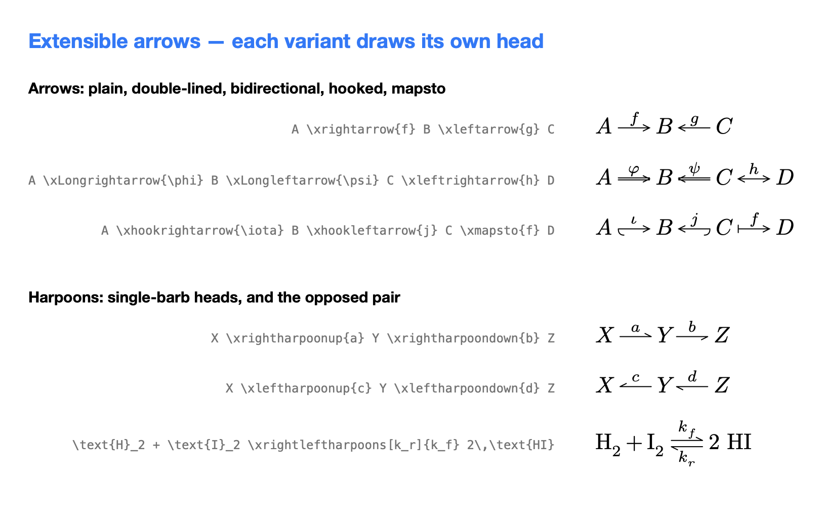
| Command | Status | Head drawn |
|---|---|---|
\xrightarrow / \xleftarrow |
✅ | Single full head, right / left |
\xLongrightarrow / \xLongleftarrow |
✅ | Double-lined shaft (⟹ ⟸) |
\xleftrightarrow |
✅ | Heads on both ends (↔) |
\xhookrightarrow / \xhookleftarrow |
✅ | Full head + hook curl at the tail (↪ ↩) |
\xmapsto |
✅ | Full head + tail bar (↦) |
\xrightharpoonup / \xrightharpoondown |
✅ | Single upper / lower barb (⇀ ⇁) |
\xleftharpoonup / \xleftharpoondown |
✅ | Single barb, left (↼ ↽) |
\xrightleftharpoons |
✅ | Two opposed stacked harpoons (⇌) |
\text{H}_2 + \text{I}_2 \xrightleftharpoons[k_r]{k_f} 2\,\text{HI}| Command | Status | Example | Note |
|---|---|---|---|
\boxed / \fbox |
✅ | \boxed{E = mc^2} |
Stroked frame with padding |
\colorbox{bg}{…} |
✅ | \colorbox{yellow}{x} |
Filled background rectangle |
\fcolorbox{border}{bg}{…} |
✅ | \fcolorbox{red}{yellow}{x} |
Filled background + stroked border |
\rule{w}{h} |
✅ | \rule{2em}{0.4pt} |
Solid filled rectangle; optional [raise] consumed |
\raisebox{s}{…} |
✅ | \raisebox{2pt}{x} |
Vertical shift of the content |
\cancel / \bcancel / \xcancel |
✅ | \cancel{x} |
Forward / backward / crossed strike over the base |
\cancelto{t}{expr} |
✅ | \cancelto{0}{x} |
Strike expr, t as a raised label |
\not |
✅ | \not=, \not\subset |
Steep slash negating the following atom |
\phantom |
✅ | \phantom{x} |
Reserves full box |
\hphantom / \vphantom |
✅ | \vphantom{\int} |
Reserves width / height only |
\smash |
✅ | \smash{\int} |
Keeps width, zero height/depth ([t]/[b] treated as plain smash) |
\mathstrut |
✅ | Invisible paren-height strut | |
\mathrlap / \mathllap / \mathclap |
✅ | Zero-width right / left / center overlap | |
\color{name}{body} |
✅ | \color{red}{x} |
Braced two-argument (localized) form |
\color{name} |
✅ | \color{red} x + y |
Stateful form — applies to the rest of the current group |
\textcolor{name}{body} |
✅ | \textcolor{#2244cc}{y} |
Named palette or #rrggbb |
Named colors: red blue green orange purple teal yellow pink magenta brown gray grey cyan black white, plus any #rrggbb hex. Scenes with explicit color
set MathScene.hasExplicitColor.
\boxed{E = mc^2} \quad \cancel{x} \quad \color{blue}{a + b} \quad \fcolorbox{teal}{yellow}{k}| Command | Status | Note |
|---|---|---|
\text / \textrm |
✅ | Upright run; interior spaces preserved (\text{if } x); nested braces kept |
\mathrm |
✅ | Upright |
\operatorname |
✅ | Upright custom operator |
\operatorname*{…} |
✅ | Upright and stacks its limits in display style (\operatorname*{argmax}_{x}) |
| Named functions | ✅ | \sin \cos \tan \log \ln \exp \lim \det \gcd \max \min … (37 total) |
Math inside \text |
✅ | \text{$n$ terms} — $…$ spans render as math (italic n, upright " terms") |
\pmod / \bmod / \pod |
✅ | a \equiv b \pmod{n} → (mod n); \bmod is a binary operator |
| Command | Status | Note |
|---|---|---|
\tag{…} |
✅ | Appended inline as body \qquad (tag) |
\tag*{…} |
✅ | Appended inline without parentheses |
\notag / \nonumber |
✅ | No-op (Vinculum does no auto-numbering to suppress) |
True flush-right tag placement is a host concern (it needs the column width); Vinculum places the tag inline after the body.
E = mc^2 \tag{1} \qquad F = ma \tag*{Newton}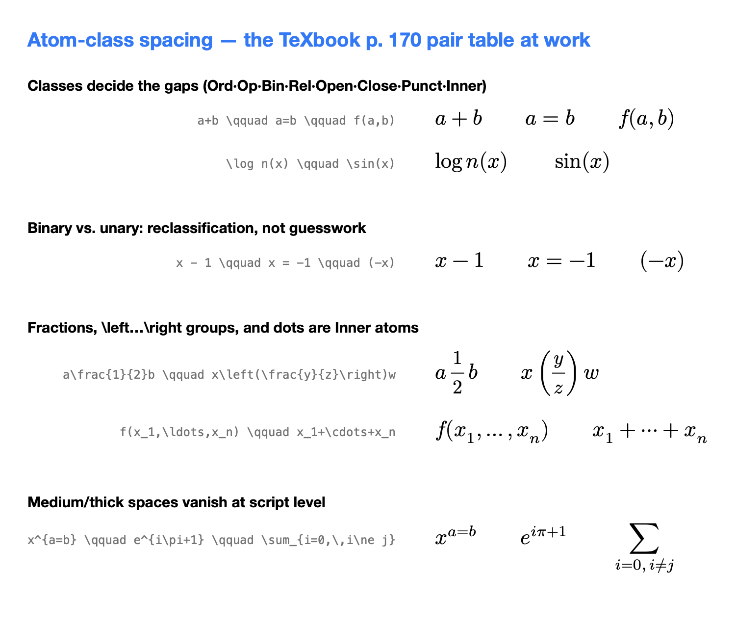
| Command | Width |
|---|---|
\, / \thinspace |
thin (3/18 em) |
\: / \> / \medspace |
medium (4/18 em) |
\; / \thickspace |
thick (5/18 em) |
\! / \negthinspace |
negative thin (−3/18 em) |
\negmedspace / \negthickspace |
−4/18 · −5/18 em |
\ (backslash-space) |
6/18 em |
\enspace |
1/2 em |
\quad / \qquad |
1 em · 2 em |
\hspace{…} / \kern… |
explicit length, default em/pt |
\mspace{…} / \mkern… |
explicit length, default mu (braced or unbraced) |
Length units understood: em, mu (1/18 em), ex (≈0.43 em), pt (1/10 em);
cm/mm/in are approximated. Negative and signed lengths are accepted.
| Command | Status | Note |
|---|---|---|
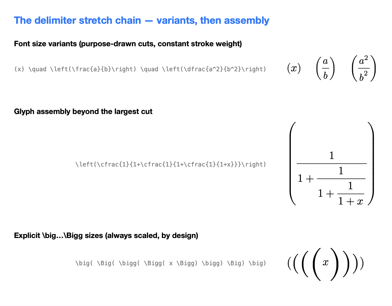
\left … \right |
✅ | Auto-sizes fences to the body: ( ) [ ], \{ \}, | \langle \rangle \lvert \rvert \lVert \Vert, \lceil \rceil \lfloor \rfloor, arrows (\uparrow \downarrow \updownarrow \Uparrow \Downarrow), \backslash, and \left./\right. for a null fence |
\middle |
✅ | \left( \frac{a}{b} \,\middle|\, c \right) — interior fence stretched to the same height, splitting the body into segments |
\big \Big \bigg \Bigg (+l/r/m) |
✅ | Enlarges the delimiter to 1.2 / 1.8 / 2.4 / 3.0× base size; the l/r/m suffix sets opening / closing / relation spacing |
The stretch chain. Every covered delimiter tries, in order: the font's
purpose-drawn size-variant glyphs (constant stroke weight), then glyph
assembly (end caps + repeatable extenders, for heights beyond the largest
cut), then point-scaling as the last resort. This runs against whichever of
the five bundled fonts is active — each font's MATH table is parsed at load.
The \big…\Bigg family always scales, deliberately: those commands request
a size, not a fit.
\left( \sum_{k=0}^{n} a_k \right) \qquad
\left\{\, x \in \mathbb{R} \;\middle|\; x > 0 \,\right\}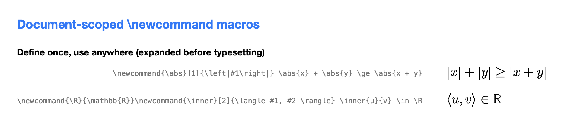
Document-scoped \newcommand / \renewcommand / \def, expanded before
typesetting. Supports #1…#9 parameters, an optional [argc], and a hard
recursion/budget cap so a self-referential macro degrades instead of hanging.
\DeclareMathOperator{\name}{text} (and the * limits form) registers a new
operator that renders like \operatorname{text} — \DeclareMathOperator{\argmax}{arg\,max}
then \argmax_x f(x).
\newcommand{\abs}[1]{\left|#1\right|} \abs{x} + \abs{y} \ge \abs{x + y}
\newcommand{\R}{\mathbb{R}}\newcommand{\inner}[2]{\langle #1, #2 \rangle} \inner{u}{v} \in \R
\DeclareMathOperator{\argmax}{arg\,max} \argmax_{x} f(x)
MathMacros.collectDefinitions(from:) scans a whole document's math segments so
a definition in one block applies everywhere; later definitions win (matching
\renewcommand).
The parsed tree is the single source of truth; three serializers read off it, so they never disagree about structure:
- Native render — CoreText (Apple), Silica/FreeType (Linux), SkiaSharp (Windows,
via the
VDL1C ABI), KotlinCanvas(Android). One platform-free layout. - SVG —
MathSVGRendereremits self-contained SVG with an embedded font, for server-side / static-site rendering (no bundled font needed at view time). MathNode.toLaTeX()— a render-equivalent LaTeX round-trip.- Presentation MathML —
MathMLExporter.export(node, display:)(orMathNode.toMathML()) serializes to<math>…</math>for accessibility trees, copy-as-MathML, and interop.<mi>/<mn>/<mo>by atom class,<mfrac>,<msubsup>,<mmultiscripts>(prescripts),<mtable>,<mover accent="true">, XML-escaped, always well-formed; unknown input degrades to<merror>.
MathMLExporter.export(MathParser.parse(#"x^2"#))
// <math xmlns="http://www.w3.org/1998/Math/MathML"><msup><mi>x</mi><mn>2</mn></msup></math>

engine.layout(node, display:, maxWidth:) wraps an over-wide equation across lines
at TeX's break points — after a binary operator or relation (+, −, =, <,
→ …), so the operator ends the line and the next term begins the next. Only the
top-level sequence breaks; nested subformulas (fractions, roots, fenced groups) stay
whole, exactly as TeX does. Lines stack baseline-aligned, the block's baseline on the
first line.
maxWidth is opt-in: omit it (or pass nil) and layout is a single line, byte-for-
byte identical to before — so nothing about existing output changes. A greedy fit
keeps each line within the budget; an unbreakable run (one wide fraction, or an atom
wider than the budget) is left intact rather than clipped.
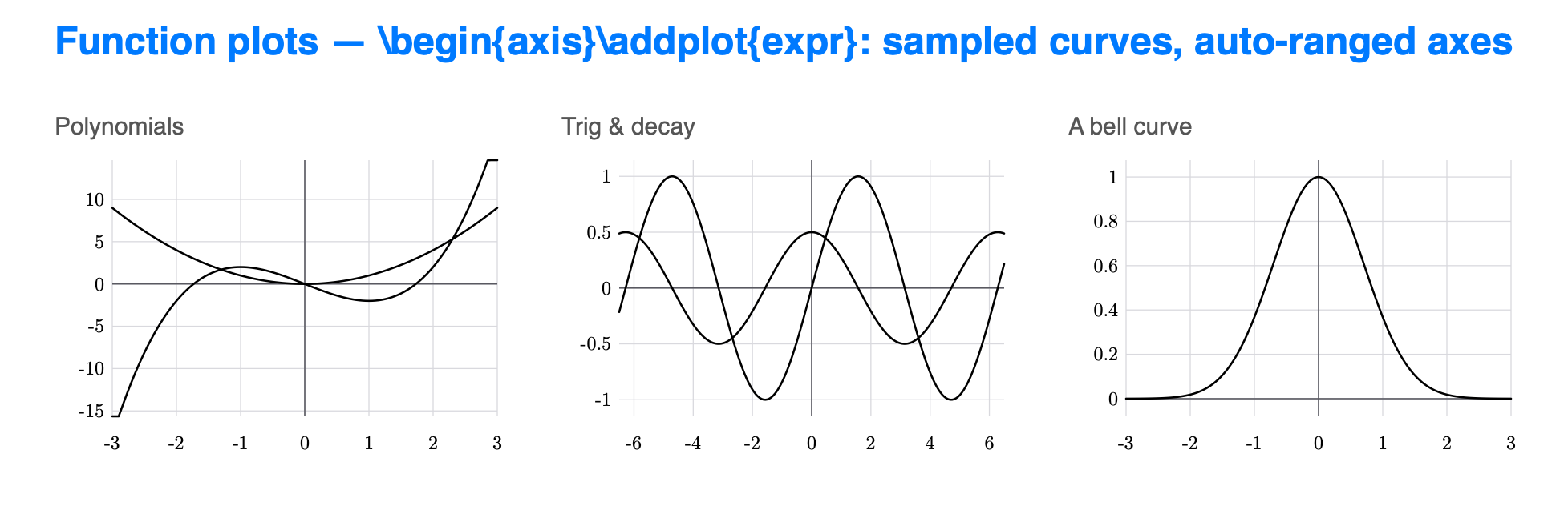
A curated pgfplots subset: \begin{axis}[domain=a:b, samples=n] \addplot{expr}; … \end{axis} (optionally wrapped in \begin{tikzpicture}). Each \addplot's expression
is sampled and drawn as a stroked curve; the axes auto-range in y, with nice-numbered
ticks and gridlines.
The expression evaluator (MathExpression) handles + - * / ^, unary minus,
parentheses, the variable x, constants pi/e, and the functions sin cos tan exp ln log sqrt abs sinh cosh tanh atan floor ceil.
\begin{axis}[domain=-3:3, samples=200] \addplot{exp(-x^2)}; \end{axis}Scope: this is a focused plotting feature, not full pgfplots/TikZ — arbitrary TikZ
graphics remain out of scope. Everything is stroked paths + glyph runs, so a plot
renders identically on every platform through VDL1.
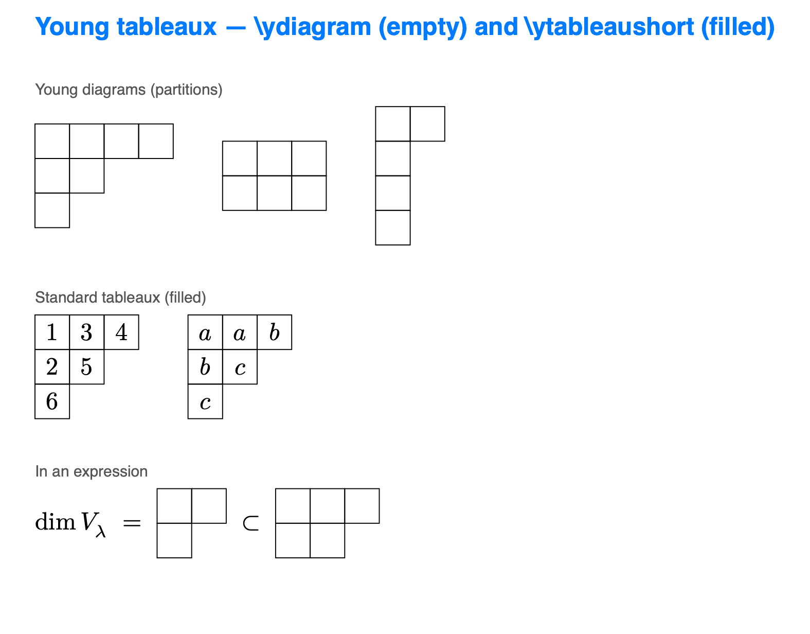
\ydiagram{4,2,1}— an empty Young diagram; the partition gives each row's length.\ytableaushort{134,25,6}(also\young(…)) — a filled tableau; each atom is a cell,,starts a new row,{…}is a multi-token cell.
A grid of bordered square cells (drawn as stroked paths), left-aligned and stacked
top-down — usable inline in an expression (\dim V_\lambda = \ydiagram{2,1}). Renders
on every platform through VDL1; round-trips through toLaTeX.
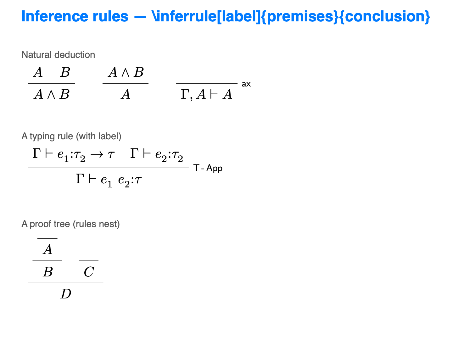
\inferrule[label]{premises}{conclusion} (aliases \infer, \prftree) typesets a
natural-deduction rule: the premises are centered in a row above a horizontal bar, the
conclusion is centered below, and the optional bracketed label sits at the bar's right at
script size.
- Premises are separated by
\\; an empty group (\inferrule{ }{A}) is an axiom (bar with nothing above it). - Rules nest — a premise can itself be an
\inferrule, so full derivation trees build bottom-up (\inferrule{\inferrule{A}{B} \\ C}{D}). - Labels accept mathpartir's
[left=Name]spelling; thekey=is dropped, the value is typeset.
The bar sits on the math axis and spans the wider of the two rows, so rules line up when
stacked. Drawn as a rule() primitive plus centered sub-scenes — renders on every platform
through VDL1, speaks as "from …, and …, infer …", and exports to MathML as a
zero-numerator <mfrac>.
\inferrule[\mathsf{T\text{-}App}]
  {\Gamma \vdash e_1 : \tau_2 \to \tau \\ \Gamma \vdash e_2 : \tau_2}
  {\Gamma \vdash e_1\ e_2 : \tau}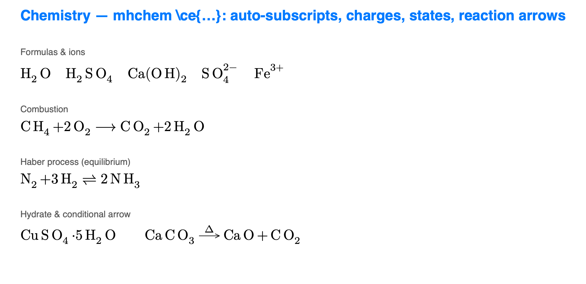
\ce{…} typesets chemical formulas and equations. Implemented as a transpiler to
LaTeX (MHChem.transpile), so it reuses the whole engine — no chemistry-specific
layout. Covers:
- Auto-subscripts:
\ce{H2O}→ H₂O,\ce{H2SO4}→ H₂SO₄. - Groups:
\ce{Ca(OH)2}→ Ca(OH)₂ (subscript after the group). - Charges:
\ce{SO4^2-}→ SO₄²⁻,\ce{Fe^3+}→ Fe³⁺. - Coefficients:
\ce{2H2 + O2}→ a leading number is stoichiometric, not a subscript. - Reaction arrows:
->,<-,<->,<=>(equilibrium ⇌), and conditional->[\Delta](drawn as\xrightarrow). - Bonds:
=(double),#(triple ≡); states(s) (l) (g) (aq); hydrate*→ ·.
\ce{N2 + 3H2 <=> 2NH3} \qquad \ce{CaCO3 ->[\Delta] CaO + CO2}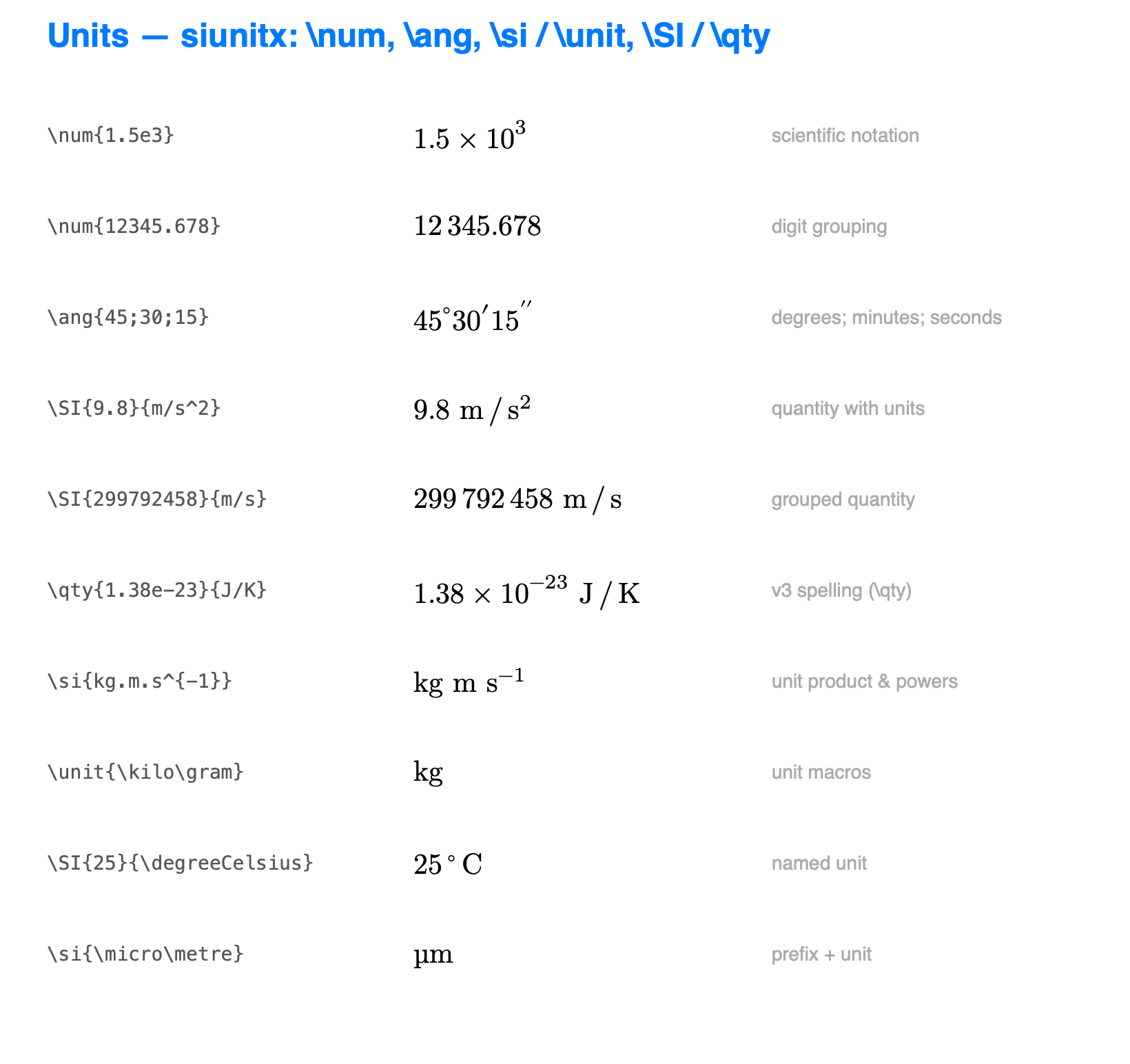
Physical quantities and units, the same transpiler approach as mhchem
(SIUnitx): each command expands to LaTeX and reuses the whole engine — no
units-specific layout. Both siunitx v2 and v3 spellings are accepted.
\num{…}— a number:\num{1.5e3}→ 1.5×10³ (scientific notation),\num{-3.2e-4}, and thin-space digit grouping every three digits once a part has ≥5 digits (\num{299792458}→ 299 792 458).\ang{…}— an angle:\ang{45}→ 45°,\ang{45;30;15}→ 45°30′15″ (degrees; minutes; seconds).\si{…}/\unit{…}— units only. Literal symbols (kg.m.s^{-1}) or macros (\kilo\gram,\metre\per\second\squared);./~are inter-unit thin spaces,/a solidus,^a power,\per/\squared/\cubedthe usual operators. Recognizes SI prefixes and base/derived units, with special glyphs upright (µ, Ω, Å, °C).\SI{…}{…}/\qty{…}{…}— a number and a unit, thin-spaced:\SI{9.8}{m/s^2},\qty{1.38e-23}{J/K}.
Unknown unit macros pass through as real commands, so nothing is silently dropped.
\SI{9.8}{m/s^2} \qquad \qty{1.38e-23}{J/K} \qquad \ang{45;30;15}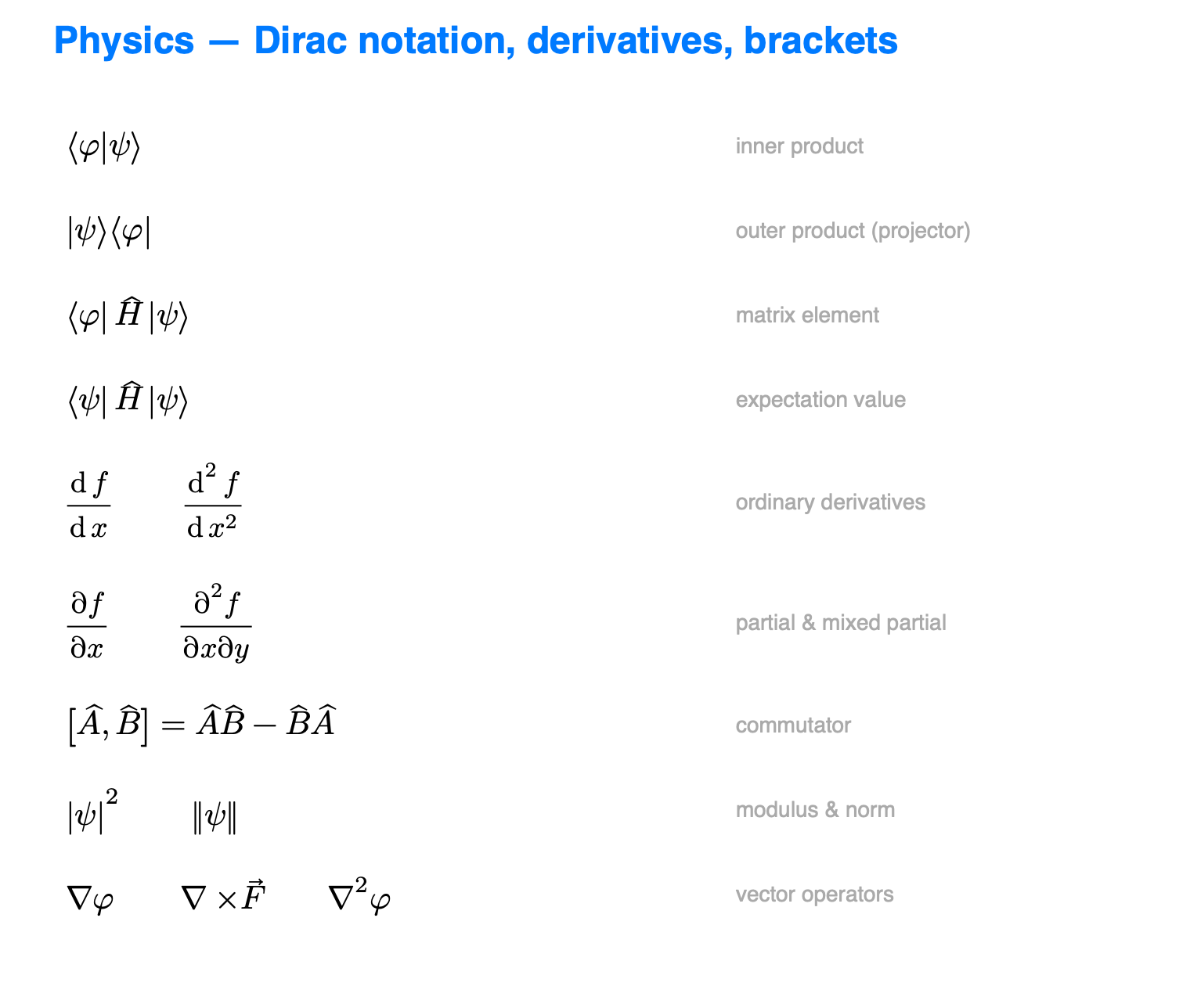
The physics package's most-used macros, again a transpiler (Physics): each
expands to LaTeX (auto-sizing \left…\right, fractions, upright \mathrm) and reuses
the whole engine.
- Dirac notation —
\bra{ϕ}→ ⟨ϕ|,\ket{ψ}→ |ψ⟩,\braket{ϕ}{ψ}→ ⟨ϕ|ψ⟩ (single-argument\braket{ψ}→ ⟨ψ|ψ⟩),\ketbra{ϕ}{ψ}→ |ϕ⟩⟨ψ|,\expval{A}{ψ}→ ⟨ψ|A|ψ⟩,\mel{ϕ}{A}{ψ}→ ⟨ϕ|A|ψ⟩. Aliases:\ip/\innerproduct,\op/\outerproduct,\ev,\matrixel. - Derivatives —
\dd{x}→ dx (upright d),\dv{f}{x}→ df/dx,\dv[2]{f}{x}→ d²f/dx²,\pdv{f}{x}→ ∂f/∂x,\pdv{f}{x}{y}→ ∂²f/∂x∂y (mixed). - Brackets —
\abs{x}→ |x|,\norm{v}→ ‖v‖,\comm{A}{B}→ [A, B],\acomm{A}{B}→ {A, B},\order{x}→ O(x). - Vector operators —
\grad→ ∇,\curl→ ∇×,\laplacian→ ∇²,\Tr/\tr,\rank. (\divis deliberately left as the core division sign ÷.)
\comm{\hat{A}}{\hat{B}} = \hat{A}\hat{B} - \hat{B}\hat{A} \qquad
\pdv{f}{x}{y} \qquad \braket{\phi}{\psi}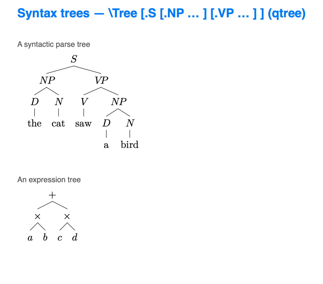
\Tree [.S [.NP … ] [.VP … ] ] (qtree / tikz-qtree syntax; \qtree is an alias)
typesets a syntax or parse tree: a labelled root centered above its children, joined by
straight edges.
- Each
[.Label child … ]is an internal node;.Labelis the node label, and every child is either another[.… ]or a bare leaf (a word or terminal). - Multi-token labels/leaves use a group:
[.{NP} \text{the cat} ]. - Labels are arbitrary math, so expression trees work too:
\Tree [.{+} [.{\times} a b ] c ].
A real 2D tidy-tree layout — subtree widths computed bottom-up, nodes placed
top-down with parents centered over their children, edges drawn as stroked paths. New
MathNode.syntaxTree; renders identically on all five platforms through VDL1,
round-trips through toLaTeX, and speaks its structure.
\Tree [.S [.NP [.D \text{the} ] [.N \text{cat} ] ]
          [.VP [.V \text{saw} ] [.NP [.D \text{a} ] [.N \text{bird} ] ] ] ]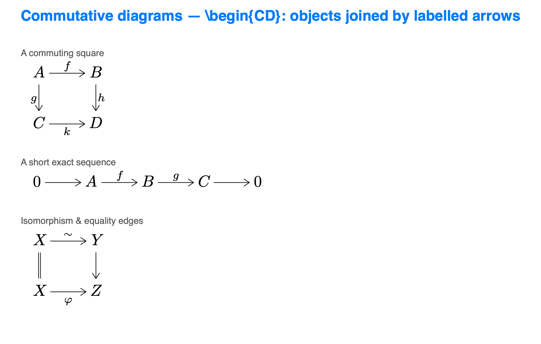
\begin{CD} … \end{CD} (amscd): objects on a grid joined by labelled arrows.
| Connector | Meaning |
|---|---|
@>a>b> / @<a<b< |
horizontal arrow → / ←, a above, b below |
@VaVbV / @AaAbA |
vertical arrow ↓ / ↑, a left, b right |
@= / @| |
a horizontal / vertical equality edge (double rule, no head) |
@. |
no arrow (an empty connector) |
\begin{CD}
A @>f>> B \\
@VgVV @VVhV \\
C @>>k> D
\end{CD}
Arrows are drawn as stroked paths (shaft + chevron head) and labels are laid out
at script size, so a diagram renders identically on every platform through the VDL1
wire — no diagram-specific primitive. Round-trips verbatim through toLaTeX.

Document-scoped, like macros — MathText.attributedString(from:numberEquations:):
\tag{…}/\tag*{…}set an equation's number explicitly (already placed inline).\label{key}records the number of the equation it sits in;\eqref{key}resolves to(N)and\ref{key}toN, throughout prose and math. A dangling key renders(?), so a broken reference is visible.- With
numberEquations: true, display equations that neither\tagnor\notagauto-number sequentially. It's opt-in: by default nothing is auto-numbered (so$$…$$stays unnumbered, matching LaTeX).\notag/\nonumbersuppress a number;\label,\notag,\nonumberare stripped before the equation renders.
\[ E = mc^2 \label{eq:e} \]        % (1) when numberEquations: true
As shown in \eqref{eq:e}, …        % → As shown in (1), …
The numbering/label logic lives in MathNumbering (platform-free, headless-tested);
MathText applies it during document rendering.
Honest list of what degrades to a source fallback (or is only partially honored):
- Out of scope by design:
\href,\includegraphics, siunitx,\verb, and general TikZ graphics (a curated pgfplots subset is supported — see "Function plots" above — but arbitrary\draw/\node/\pathpictures are not). \mathcal/\mathfrak/\mathscrrender letters only (no digit variants exist in Unicode).- Old-style
\rm/\it/\sl/\mitswitches render, but round-trip through\mathrm/italic so their exact spacing may shift on re-serialization; the alphabet switches (\bf/\cal/\frak/\bb/\scr/\sf/\tt) round-trip exactly. \displaylimitsis accepted and is a no-op — it restores the current style's default placement, which an unmodified operator already uses. (\limitsand\nolimitsboth actively force their form and round-trip exactly.)- A bare
\\outside an environment is a no-op (an explicit forced break). Automatic width-aware breaking is available vialayout(node, maxWidth:)— see "Automatic line breaking" above.
If you need one of these, it's a good first contribution — see the "add a command" walkthrough in ARCHITECTURE.md.